Nearest Neighbor Distribution
Applicability


When the Compute Nearest Neighbor Distribution option is active, two values are computed by the code automatically: the Mean Nearest Neighbor Separation Distance and the Nearest Neighbor Separation Distance Probability Distribution Function. These are both useful metrics when characterizing particle dispersions. The Particle Output Data page describes the output for this option.
For additional information, see the associated tutorial video.
Mean Nearest Neighbor Separation Distance
The mean nearest neighbor separation distance, \(\langle r_{nn} \rangle\), is the ensemble-averaged distance between each particle and its nearest neighbor:
where \(r_{nn}\), the nearest neighbor separation distance of an individual particle and \({N}\) is the total number of particles in the ensemble. Both \(r_{nn}\) and \(\langle r_{nn} \rangle\) are frequently normalized by the Wigner–Seitz radius:
where \({V}\) is the total volume of solids. Physically speaking, \(a\) represents the mean available volume per particle. A ratio \({{\langle r_{nn} \rangle}}/a<<1\) implies poor particle dispersion, such that particles are (on average) not occupying the full available system volume.
In Figure 1, we present the time-evolution of \(\langle r_{nn} \rangle\) for an ensemble of particles added to an agitated vessel containing. The Wigner–Seitz radius, calculated from Equation 1, is shown in the figure. As particles disperse through the system, \(\langle r_{nn} \rangle\) advances a final quasi-steady state value that fluctuates near \(a\). The initial value of \(\langle r_{nn} \rangle\) is informed by the initial packing density of the particle within the injection geometry. The time required for \(\langle r_{nn} \rangle\) to approach \(a\) represents a dispersion time scale and is typically informed by the simulation blend time.
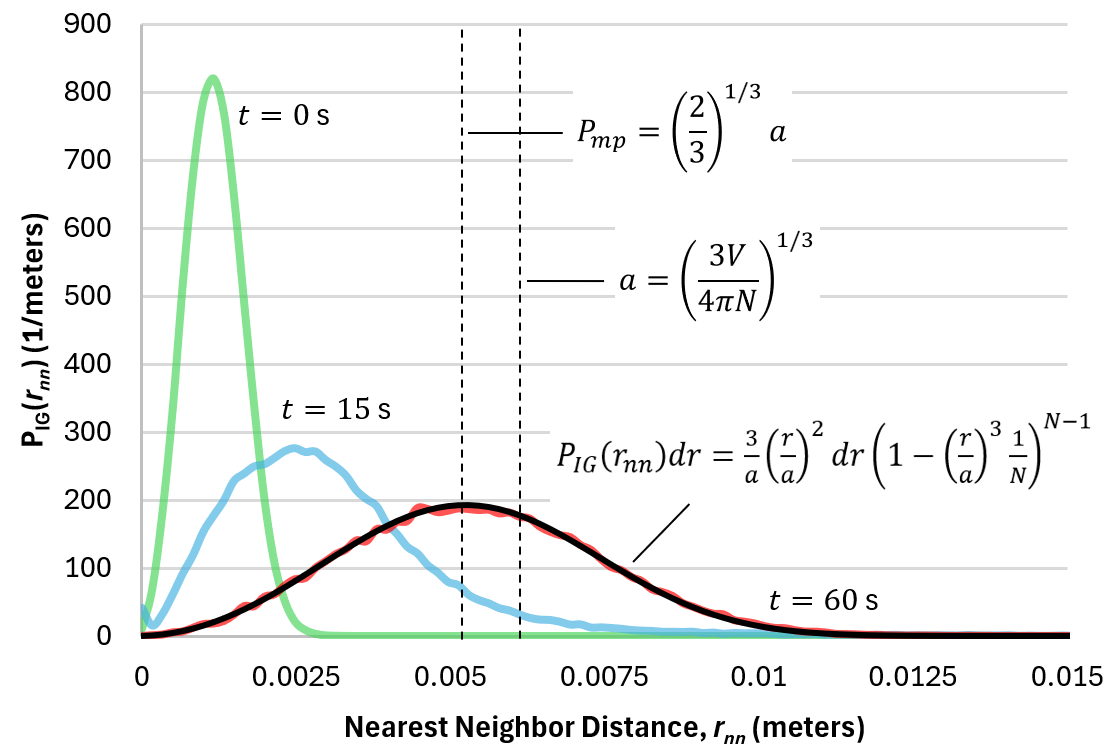
Fig. 76 Figure 1
Nearest Neighbor Separation Distance Probability Distribution Function
The nearest neighbor separation distance probability distribution function, \(P(r_{nn})\), characterizes the distribution of \(r_{nn}\) for an ensemble of particles. That is, rather than reducing the entire set of nearest neighbor distances into a single ensemble mean, \(P(r_{nn})\) illustrates the distribution of \(r_{nn}\) across the ensemble. This distribution can be compared to nearest neighbor distribution function of non-interacting ideal-gas gas molecules,
where \(a\) is the Wigner–Seitz radius defined above. This distribution comes from kinetic theory and efforts to describe the spatial distribution of ideal gas molecules across a volume. The distribution is not a delta function; a random distribution across space means that some particles will be closer to their nearest neighbor than other particles are to their nearest neighbor. Moreover, the distribution is not symmetric, as the most-probable nearest neighbor separation distance is \(\left( \frac{2}{3} \right)^{\frac{1}{3}} a\). This behavior stems from the physical requirement that all nearest neighbor distances must be positive.
In Figure 2, we present the time-evolution of \(P(r_{nn})\), for an ensemble of 10,000 particles added to an agitated vessel containing 0.095 \(m^3\) of fluid. This is the same data used to generate the data presented in Figure 1. Following injection, the distribution is narrow and the most probable \(r_{nn}\) is small compared to \(a\). This initial distribution, as discussed above, is informed by the initial packing density of the particle within the injection geometry. As particles disperse through the system, \(P(r_{nn})\) broadens and accesses a larger domain of \(r_{nn}\) values. Eventually, as the particles become fully dispersed, \(P(r_{nn})\) recovers the a priori expectations from Equation 3. The time required for \(P(r_{nn})\) to approach \(P_{IG}(r)\) represents a dispersion time scale and is typically informed by the simulation blend time.
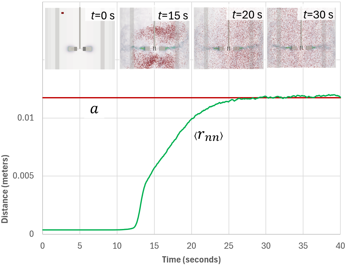
Fig. 77 Figure 2.0