Modeling Inlet and Outlet Boundary Conditions
Boundary Condition Overview
In fluid dynamics, the governing equations cannot be solved without specifying additional information at the boundaries of the domain. Constraints must be imposed at the domain limits to obtain a unique, physically meaningful solution. The boundary conditions are the constraints applied at the edges of the computational domain to define how the fluid behaves.
From this definition, we understand that a boundary condition prescribes one or more flow variables (such as velocity, pressure, species concentration, or temperature) on the surface enclosing the fluid domain. In general, boundary conditions fall into three main categories:
Dirichlet: Value Boundary Condition -> Specifies the value of a fluid variable
Neumann: Gradient Boundary Condition -> Specifies the gradient of a variable
Robin: Mixed Boundary Condition -> Specifies a combination of value and gradient
In M-Star, we primarily use Dirichlet and Neumann boundary conditions. Although boundaries can be defined as walls (no‑slip, slip, adiabatic, etc.) or as inlets and outlets, in this document we will focus on inlet and outlet boundary conditions—how to create them, the different types available, and the best practices for their effective use.
For further details regarding wall boundary conditions, please visit the Main Lattice and Static Body pages.
Inlet and Outlet Boundary Conditions
Inlet and outlet boundary conditions determine how the flow enters and leaves the fluid domain. These boundary conditions can be defined by prescribing velocity, pressure, or flow rate, among other variables. For a detailed explanation of the available inlet and outlet boundary conditions, see Boundary Condition Types.
Create Inlet and Outlet Boundary Conditions
To create inlets and outlets, we use the Create function in M‑Star Pre under Fundamentals, where you can choose a Static Inlet/Outlet or a Moving Inlet/Outlet.
From this point forward, we will focus exclusively on Static Inlet and Outlet Boundary Conditions, as they are the most used and offer a wider range of configuration options.
To create a static inlet or outlet boundary condition, select Create and then choose Static Inlet/Outlet. This action adds a new item to the Model Tree and opens the Inlet/Outlet Setup form. This form allows you to choose the boundary where the condition will be applied:
Point on bounding box
You can place a point anywhere on the bounding box to select the corresponding region as an inlet or outlet. If multiple boundaries lie on the same bounding box face, the software automatically detects the distinct regions defined by the geometry. You can then click within the desired region to select it while excluding the others. This method allows you to define multiple boundary conditions on a single bounding box face.
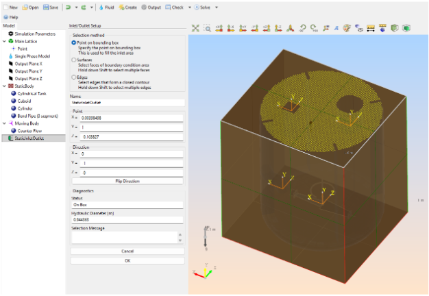
Selection Method: Point on Bounding Box
Surface
Select the surface directly from the geometry where you want to apply the inlet or outlet boundary condition by clicking on the desired face (hold Shift to select multiple surfaces). When this option is chosen, a dialog box appears that allows you to filter which geometric elements should be considered during selection. This is especially helpful for large or complex geometries where inlet or outlet surfaces may be hidden or embedded within other components.
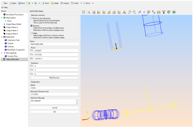
Selection Method: Surfaces
Edges
Select the edges in the geometry that form a closed contour (hold Shift to select multiple edges). If no face exists for the selected contour, M-Star will automatically generate one to close the control volume. As with the surface selection method, a filtering dialog will appear to help refine which geometric elements are considered during selection.
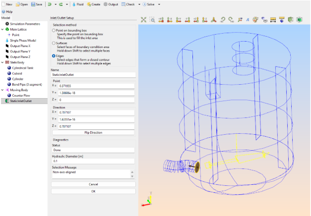
Selection Method: Edges
Once the inlet or outlet has been created, all of its characteristics can be configured through the options in the Property Grid—including boundary condition type, magnitude, operation duration, and more. Whether the boundary condition functions as an inlet or an outlet depends on how these parameters are defined.
If, for example, the boundary condition type is set to Velocity and the direction vector points into the control volume, the boundary acts as an inlet, since fluid enters the domain. If the direction is reversed—pointing outward from the control volume—the boundary acts as an outlet. This logic applies broadly to velocity and flow-rate boundary conditions.
Some boundary condition types are restricted by design: certain options can only be used as inlets (such as inlet single-pulse, inlet multi-pulse, and recirculation return), while others can only be used as outlets.
Guidelines and Recommendations
Physical Definition
As a general guideline, inlets and outlets should be defined using realistic physical properties, such as velocity, pressure, or flow rate. Whenever possible, they should be positioned far from regions of strong disturbances to minimize backflow or artificial acceleration effects.
For single-phase simulations, maintain mass or volume balance within the system—because volume is conserved, the total inflow must equal the total outflow. In practical terms, defining an inlet requires defining at least one outlet to satisfy mass continuity. If the mass is not conserved, the LB density will increase or decrease, leading to an incorrect solution or simulation divergence.
Static vs. Moving Boundaries
When using a Static Inlet/Outlet boundary condition, it must always be applied to a static body. It should never be assigned to a moving body. If a moving boundary is required, the Moving Inlet/Outlet option must be used.
On-Lattice Placement
Whenever possible, align inlets and outlets with the lattice (on-lattice boundary condition) when using lattice-based boundary conditions. An on-lattice boundary condition is a boundary treatment where the physical boundary aligns exactly with lattice nodes or links, allowing boundary conditions to be applied locally without interpolation. Geometrically, an on-lattice boundary condition is one where the boundary surface coincides with lattice planes, has normals aligned with the Cartesian lattice axes, and does not cut through lattice voxels or links at arbitrary angles. This improves numerical stability, enhances boundary resolution, reduces noise and artifacts, and ultimately leads to more accurate and realistic simulation results. Ensure that inlet and outlet regions are sufficiently resolved—typically with at least 10 lattice points across each opening—to avoid poorly captured boundary behavior.
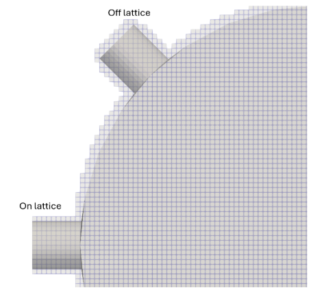
The image above illustrates how volume discretization affects off-lattice boundary conditions. Because of the discretization, the off-lattice inlet exhibits a stair-step pattern on both the pipe walls and the inlet surface. This reduces the effective boundary-condition area from 10 voxels across in the on-lattice case to only 7 elements in the off-lattice model. As a result, the region becomes under-resolved, and the stair-step geometry leads to poor wall representation. This, in turn, impacts local mass and velocity fields, as well as the overall flow rate.
Strategies for Unavoidable Off-Lattice Boundaries
The most reliable way to obtain an on-lattice boundary condition is to reposition the geometry so the boundary aligns with one of the main lattice axes. However, this is not always feasible, and some boundaries must remain off-lattice (for example, a vessel with two inlets rotated 45 degrees). In such cases, several strategies can help improve simulation quality:
Increase lattice refinement to boost the number of voxels across the boundary surface and reduce the stair-step effect.
Extend the inlet or outlet pipe until it intersects the bounding box. This creates a new inlet or outlet surface on the bounding box, which is inherently on-lattice.
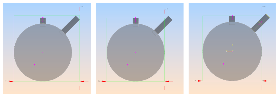
Extend the inlet or outlet pipe; intersect with the bounding box; define the boundary condition on the bounding box.
This approach can be useful for certain boundary types—particularly pressure boundaries—but may be problematic for others because the resulting inlet or outlet face becomes oblique, increasing its effective area and potentially distorting flow-rate values. Adding a pressure filter can help stabilize the inlet, though additional refinement may still be needed to further reduce stair-stepping.
For a tutorial, see On and Off Lattice Boundary Conditions.
Structural Requirements
Behind any boundary condition—whether an inlet or an outlet—there must be a solid region rather than fluid. If a boundary condition is defined with fluid on both sides, the software cannot determine which direction is “in” or “out,” leading to ambiguity and potential solver failure.
Boundary conditions can also be applied directly on the domain limits. In this case, no solid body is required behind the inlet or outlet because the back side of the boundary is not exposed to any fluid.
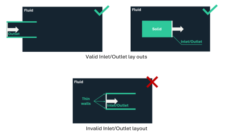
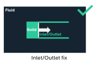
The situation described above can occur when an open cylinder is used to define an inlet—for example, when walls are needed to guide a jet of fluid. However, this setup will fail because the solver requires a solid region behind any inlet or outlet. A simple solution is to add a solid cap or body to the open cylinder, ensuring that the boundary condition is backed by solid material, as illustrated in the image below.
Numerical Stabilization Tools
Use ramp time to gradually reach the target boundary condition value. This helps prevent shocks or unphysical transients that can occur when a boundary is subjected to an instantaneous change—an effect that becomes especially significant when inlet or outlet values are large.
Use buffer length to reduce noise and instabilities in the inlet or outlet region. The buffer increases viscosity in a thin layer near the boundary, damping small-scale fluctuations and improving stability. As a guideline, start with a buffer length equal to 10% of the inlet or outlet diameter; values up to 50% are generally safe. However, the buffer should remain as small as possible because it introduces additional dissipation. If the buffer length exceeds the full inlet or outlet diameter, the simulation setup should be reviewed, as this typically indicates that some underlying assumptions are not being met.
Use pressure filters to help attenuate spurious pressure waves. These can be applied to further enhance stability.