Predicting mass transfer (kLA) in gasified bioreactors

Background

Bioreactor performance and yield is typically informed by the overall transport rate of oxygen from gas bubbles to an agitated fluid. In this work, we model a sparged, benchtop bioreactor with bubble break-up and carbon dioxide production.

Input files

Input file avaible here.

Theoretical Overview

On a bubble-by-bubble basis, convective oxygen transport from each bubble to its surrounding fluid is modeled by:

\[\dot{n}_i =H_i \left(S_i C_{g,i}-C_{f,i} \right)\]

where \(\dot{n}_i\) is the oxygen mass flux from bubble \(i\), \(H_i\) is the overall mass transfer coefficient of the bubble, \(S_i\) is the local dimensionless oxygen solubility of the fluid surrounding the bubble, \(C_{g,i}\) is the oxygen concentration in the bubble, and \(C_{f,i}\) is the the local fluid dissolved oxygen concentration. Note that when \(H_i\) is measured in m³/s and the concentrations are measured in mol/m³, the mass flux will be calculated in mol/s.

The total oxygen transfer rate, \(\dot{n}_T\), from all bubbles is then defined by:

\[\dot{n}_T =\displaystyle \sum_i^{N_b} \dot{n}_i\]

where \(N_b\) is the number of bubbles in the system.

The overall mass transfer coefficient is a function of the convective mass transfer coefficient, \(k_{L}\), and the bubble surface area, \(A\), such that:

\[H_i=k_{L,i} A_i\]

Note that \(k_{L}\) and \(A\) typically have units of m/s and m².

Dimensional analysis requires that the Sherwood number be a function of the Schmidt number and Reynolds number. [1] As such, the convective mass transfer coefficient is a function energy dissipation rate, viscosity, and Schmidt number:

\[k_{L,i} =C(\epsilon_i ν_i )^a Sc_i^b,\]

where \(\epsilon_i\), \(\nu_i\), \(Sc_i\) are the specific energy dissipation rate, kinematic viscosity, and Schmidt number of the fluid surrounding each bubble. Note that \(\epsilon_i\) and \(\nu_i\) typically have units of m²/s³ and m²/s, while the Schmidt number is dimensionless. The constants \(C\), \(a\) and \(b\) are defined from dimensional analysis and turbulence theory [2], such that

\[k_{L,i} =0.3(\epsilon_i ν_i )^{1/4} {Sc_i}^{-1/2}.\]

Note that \(k_{L}\) is typically measured in m/s.

These equations highlight the four key factors informing the oxygen transport rate:

1. concentration differences between the bubbles and the surrounding fluid,

2. number of bubbles in the system,

3. surface area of the bubbles, and

4. convective mass transfer coefficient.

From a modeling perspective, these factors identify which fluid mechanical mechanisms a numerical model must properly describe in order to correctly predict the oxygen transport rate to the fluid:

1. evolution of dissolved oxygen concentration through space and time,

2. gas bubble hold-up,

3. gas bubble size distribution, and

4. local energy dissipation rate.

A correct representation of all four individual mechanisms, along with a correct prediction of the oxygen transfer rate, indicate a mechanistically robust bioreactor model.

Modeling Overview

Within the context of lattice-Boltzmann simulations, two numerical parameters must be specified: the lattice spacing and the simulation timestep. In this section, we discuss the principles governing each parameter.

Lattice Spacing

The lattice spacing informs the smallest flow structure/eddy that can be captured by the model. In choosing a simulation resolution, we consider three intrinsic eddy length scales: the integral scale, the Taylor scale, and the Kolmogorov scale. The integral length scale, \(l\), which characterizes largest eddies in the system, is order-of-magnitude consistent with the vessel diameter:

\[l \approx T,\]

where \(T\) is the tank diameter. These eddies, which are generated by the impeller and reflect off the tank walls, are anisotropic and responsible for bulk fluid mixing and transport.

Integral scale eddies break-up and decay into increasingly smaller and isotropic (relative to the vessel diameter) structures, which eventually become converted to thermal energy by viscous dissipation. This transition from anisotropic/bulk-flow eddies into isotropic/localized eddies is characterized by the Taylor length scale \(\lambda\), defined by:

\[\frac{\lambda}{T} \approx \sqrt{\frac{15}{Re}},\]

where \(Re\) is the impeller Reynolds number.

Loosely speaking, eddies larger than the Taylor scale are anisotropic and contribute to bulk flow. Eddies smaller than the Taylor length scale are localized (relative to the vessel diameter), isotropic and contribute to micro-mixing.

Below the Taylor length scale, this eddy decay process continues down to the Kolmogorov length scale, \(\nu_k\), which describes the smallest hydrodynamic length scale in the system. The Kolmogorov length scale is also a function of Reynolds number:

\[\frac{\nu_k}{T} \approx \frac{1}{Re^{3/4}},\]

Because eddies between the Taylor and Kolmogorov length scale are short-lived and isotropic, they make limited contributions to bulk mixing and advection. They can, however, have important effects on local energy dissipation and reaction rates.

For modest Reynolds numbers up 10⁴, it is common to set the lattice spacing to the Kolmogorov length scale (the smallest eddies in the system) and run an explicit direct numerical simulation (DNS) that captures the entire turbulence spectrum. In systems with higher Reynolds numbers, such as this bioreactor, the resolution required to capture the complete turbulence spectrum (from integral down to the Kolmogorov length scale) are computationally prohibitive. Instead, large eddy simulations (LES) are applied with an eddy viscosity turbulence closure model that accounts for the effects the unresolved (sub-grid) eddies on the resolved flow field. [3]

In principle, even within an LES simulation, the lattice should be as fine as computationally practical. In practice, choosing a resolution least as fine as the Taylor length will generally sufficient to produce reliable predictions of bulk mixing and transport within turbulent systems. Although the smallest eddies are not resolved explicitly in a these simulation, their contributions to viscosity and energy dissipation automatically incorporated into the model on-the-fly by the solver. That is, the total specific energy dissipation rate (resolved plus unresolved) is used when computing \(k_{L}\).

Simulation Timestep

Since lattice-Boltzmann is an explicit solver, the simulation timestep, \(\Delta t\), is defined by the lattice spacing, the impeller tip speed, \(V_t\), and a Courant number, \(Co\), such that:

\[\Delta t = \frac{Co \Delta x}{V_t}\]

Subject to the CFL condition, the Courant number must be order-of-magnitude smaller than 1. In this work, we use a Courant number of 0.1, which is the default setting in the software.

Bubble Modeling

Bubble trajectories are governed by Newton’s second law, such that:

\[m_i \vec{a}_i=\vec{F}_{i,g}+\vec{F}_{i,a}+\vec{F}_{i,p}+\vec{F}_{i,D}\]

where \(m_i\) and \(\vec{a}_i\) represent the mass and acceleration vector of bubble \(i\), \(\vec{F}_{i,g}\) is the net gravity force (gravity plus buoyancy), \(\vec{F}_{i,a}\) is the added mass force, \(\vec{F}_{i,p}\), is the pressure gradient force, and \(\vec{F}_{i,d}\) is the drag force with a literature drag coefficient. [4] Particles are two-way coupled to the fluid via Newtons third law, such that a body force, \(\vec{F}_{f,j}\):

\[\vec{F}_{f,j}=-\left(\displaystyle \sum_i^{i \in j} \vec{F}_{i,g}+\vec{F}_{i,a}+\vec{F}_{i,D} \right)\]

is superimposed on the fluid voxel \(j\) containing the set of bubbles \(i \in j\). Note that this fluid body force does not include the pressure gradient force on the particle, as this force is already incorporated into the Navier-Stokes equations.

Bubble coalescence is likewise modeled directly via bubble-bubble interactions. To determine whether two colliding bubbles coalescence or bounce, we calculate the approach Reynolds number:

\[Re_a=\frac{U_a d_h}{\nu}\]

where \(U_a\) is the approach velocity and \(d_a\) is the harmonic mean diameter of the bubble pair:

\[d_a=\frac{2d_{i1}d_{i2}}{d_{i1}+d_{i2}},\]

where d_{i1} and d_{i2} are the diameters of the two interacting bubbles.

When \(Re_a\) exceeds the critical Reynolds number of 40, the bubbles coalesce to create a new bubble while conserving volume total. If \(Re_a\) is less than 40, the bubble pair undergoes an elastic bounce. [5]

Bubble break-up occurs at the level of individual bubbles and is driven by the local energy dissipation rate. From first-principles turbulence theory, the equilibrium bubble size represents a balance between shear and surface tension forces, such that: [2]

\[D_e \approx \frac{ \sigma^{\frac{3}{5}}}{ \rho^{\frac{3}{5}} \epsilon^{\frac{2}{5}}}\]

where \(\sigma\) is the bubble-to-liquid surface tension and \(\rho\) is the fluid density.

If a bubble enters a region wherein \(D_e\) is smaller than the current bubble diameter, a break-up event is very likely to occur. During this break-up event, the bubble is split into randomly sized daughter particles in a manner that conserves total volume. As discussed below, various break-up models can be tested.

Species Transport

Dissolved oxygen transport within the vessel is modeled via the advection-diffusion-reaction equation:

\[\frac{d c_j}{dt} = \nabla \cdot D \nabla c_j + \nabla \cdot \left( \vec{v}_j c_j \right) +\frac{\dot{n}_j}{V}\]

Where \(c_j\) is the dissolved oxygen concentration in fluid voxel \(j\), \(D\) is the dissolved gas diffusion coefficient, \(\vec{v}_j\) the fluid velocity vector at voxel \(j\), \(V_j\) is the volume of the fluid voxel, and \(\dot{n}_j\) is the oxygen mass transfer rate between the bubbles contained in fluid voxel \(j\) and the fluid inside the voxel. This source term can be recast as:

\[\dot{n}_j= \displaystyle \sum_i^{i \in j} k_{L,i} A_i \left( S_j C_{g,i}-C_{f,i} \right),\]

where \(i\) denotes bubble properties and \(j\) denotes fluid voxel properties.

If the bubbles have similar oxygen concentrations and are small compared to the lattice spacing, these equations can be combined as:

\[\frac{d c_j}{dt} = \nabla \cdot D \nabla c_j + \nabla \cdot \left( \vec{v}_j c_j \right) +k_{L,j} a_j \left( S_j C_{g}-C_{f,i} \right),\]

were \(a_j\) is the specific surface area of the bubbles in voxel \(j\), measured in units of 1/m. The units on \(k_{L,j} a_j\) are 1/s. This parameter, as discussed below, is called the volumetric mass transfer coefficient and can be measured experimentally.

The framework presented here is general and presents only a minimal set of adjustable parameters. Inasmuch as the vessel is turbulent, the \(k_{L}\) relationship does not change with system length scale and is not adjusted between simulations. The forces governing bubble transport are likewise set a priori from first principles and are not adjusted between simulations or length scales. Similarly, the critical Reynolds number for break-up is determined from a priori experimental observation, and likewise is not tuned between models or by system size. Although the simulation resolution and time-step must be defined, this value can be anchored to the intrinsic turbulent length scale and convergence can be tested.

A bubble break-up model must be selected, a point we explore below. Differences between the various break-up kernels were small, however, suggesting that the ability to break-up (in this system) is more important than the exact shape of the distribution function. This minimization of the number of adjustable parameters is crucial if we are to develop a robust, physically grounded reactor model.

Building the Model

Tank and impeller assembly follow the typical geometry import procedures. The impeller diameter is 0.058 m and, as shown in klaLabel111, is positioned at the center of a 0.18 m-diameter tank. The bottom of the shaft is located 0.05 m above the bottom of the tank. The impeller speed is set to 400 RPM, which corresponds to a tip speed of 1.23 m/s. A free surface model was selected, with the fluid density and viscosity set to 1000 kg/m³ and 10^-6 m²/s. The initial fluid volume was set to 3.9 L. A small 0.02 m headspace was specified, which is sufficient to account for any sloshing or vortex formation.

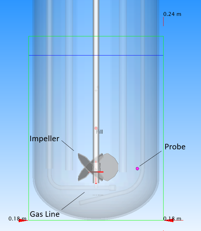
Geometry of the 3.9 L bioreactor

The Reynolds number of this impeller is 23,000, which corresponds to a Taylor length scale of 4.5 mm and a Kolmogorov length scale of 90 µm. We choose a lattice spacing of 1 mm, which is conservative relative to the Taylor length scale and will capture the anisotropic eddies responsible for bulk mixing and transport. The smaller (anisotropic) eddies between this lattice spacing and the Kolmogorov length scale are incorporated into an eddy viscosity via the large eddy closure model. Contributions from these sub-grid eddies to the total energy dissipation rate are calculated on-the-fly and incorporated into the mass transfer coefficient expressions.

We select the default Courant number of 0.1 that, for the lattice spacing and tip velocity here, corresponds to a simulation timestep of 79 µs.

In both experiment and simulation, bubbles enter the system via seven, 0.8-mm diameter openings positioned on the bottom of the gas line directly below the impeller. The gas flow rate was set to 0.4 L/min. The initial bubble diameter set to 1.1 mm, a value motivated by the work of Geary and Rice [6]. We consider the gravity, buoyancy, free particle drag and added mass forces on the bubbles. Newton’s third law is evoked to model fluid-bubble coupling. Coalescence is enabled using the default critical Reynolds number of 40.

A coalescence start time of 2 seconds and sampling interval of 5 timesteps were selected. These start time and sampling intervals were selected to (i) ensure smooth start-up and (ii) maximize runtime performance by reducing the frequency of bubble neighbor distance calculations.

A dissolved oxygen field is defined with an initial background concentration of 0 mol/L and a diffusion coefficient of \(2 \times 10^{-9}\) m²/s. A static probe is placed between the impeller and the tank side wall. The initial bubble oxygen volume fraction is set to 1.0, meaning the injected bubbles are pure oxygen. The molar volume of the oxygen is set to 0.0224 m³/mol, a value derived from the ideal gas law. Note that this molar volume corresponds to a oxygen concentration of 0.0446 mol/L (\(=\frac{1}{22.4}\) mol/L). The dimensionless solubility of oxygen is taken to be 0.032. [7]

Motivated by the expressions defined above, the mass transfer coefficient is written as:

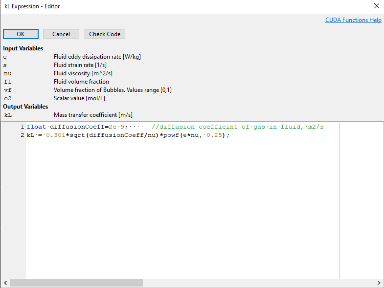
Per the transport relations defined above, the scalar coupling is then written as:

Four key points are worth noting:

1. The bubble \(k_L\) is computed on-the-fly internally by the solver for each bubble using the expression defined by the user.

2. The bubble area is computed on-the-fly internally by the solver for each bubble. This expression automatically accounts for changes in the bubble area of each bubble due to break-up or coalescence.

3. The species concentration in the bubble is calculated and updated automatically in the solver. For single gas systems like this, the oxygen concentration will remain constant at 0.0446 mol/L. For multi-species systems (see below), changes in the bubble composition will updated automatically.

4. Species leaving/entering the bubble will cause the bubble to shrink/grow. Changes in the bubble volume are linked to mass transfer using the molar volume.

Running the Model

The simulation was executed on a desktop Nvidia V100 GPU. 60 seconds of runtime were achieved in about 1 hour of wall time. Output data and slices were saved every 0.05 seconds. Volume data was saved every 2 seconds.

Analyzing the Output

A movie of the simulation output for a model with no bubble break-up is presented below. We observe gas bubbles entering the system through the sparge, then coalescing in the body of the tank to form an equilibrium bubble size distribution before leaving through the free surface. We observe turbulent fluid motion around the impeller and see the decay in turbulence as fluid moves up the wall toward the top of the tank. The maximum velocity is consistent with the impeller tip speed. The free surface is mostly flat, with a small vortex near the spinning shaft. The two-phase flow field becomes steady after just a few seconds. We also observe the dissolved oxygen concentration increasing within the fluid over this period.

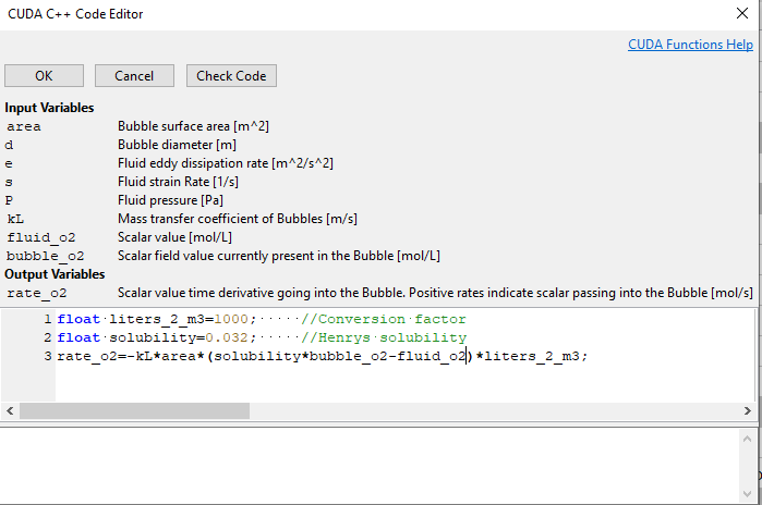
In klaLabel1 we compare the shaft power to the total power dissipation. This data comes directly from the thermodynamics.txt output file. Note that this dissipation includes both resolved and unresolved components of the energy dissipation.

The shaft power is computed from the torque on the impeller. The steady state power draw corresponds to power number around 1.5. This value is consistent with the measured value for wide-blade pitch blade turbines, and reasonable given the topology of the tank internals. The total power dissipation represents the volume total energy dissipation across the fluid.

At steady state, the shaft power is consistent with the total fluid dissipation (within 5-10%). This behavior is expected and indicates that the code is satisfying the first law of thermodynamics. The consistency between the predicted power number, measured values for similar impellers, and the total power number gives confidence that the local energy dissipation rates used to compute mass transfer rates are valid. Note that the additional 0.02-0.05 W dissipation beyond that shaft power is consistent with the additional power dissipation caused by the rising bubbles. To an order-of-magnitude, the additional dissipation expected from the bubbles is equal to the gas flow rate times the hydrostatic pressure head at the bottom of the vessel.

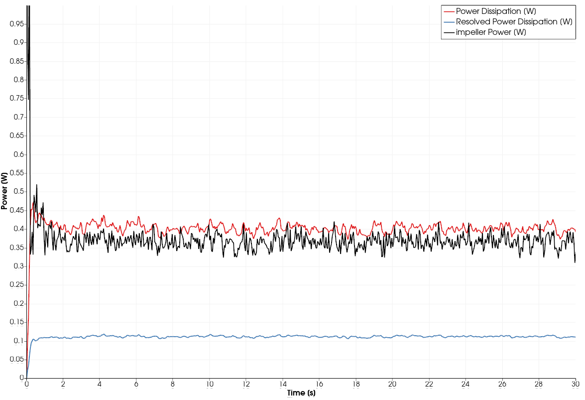
Power input and dissipation within the vessel

In klaLabel2, we present a snapshot of the bubble size distribution during steady state operation. The mean bubble size above the impeller is around 3 mm—a value consistent with measurement. [] The largest bubbles approach 6 mm in diameter, while the smallest bubbles are those that enter the system through the sparge. Recall that, in this model, break-up is deactivated.

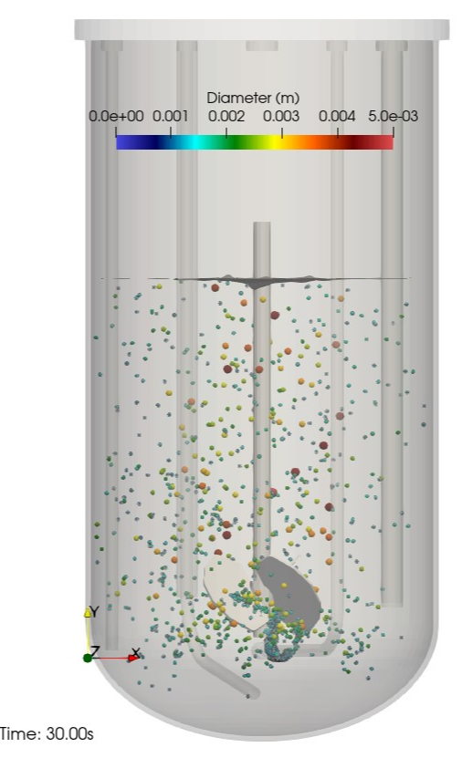
Bubble size distribution in the bioreactor

In klaLabel3, we present the time-evolution of the dissolved oxygen concentration, as measured at the probe location. This data comes directly from the probe.txt output file. The gas bubbles enter the system as pure oxygen. As discussed, per the ideal gas relationship, the oxygen concentration is taken to be 0.0446 mol/L. The non-dimensional solubility is set to 0.032. With these properties, the saturated oxygen concentration in the fluid will be 0.0014 mol/L.

After only 60 seconds of runtime, the oxygen concentration has not yet approached the saturation limit. However, the volumetric mass transfer coefficient (\(k_L a\)) at the probe can still be extracted from the time-evolution of the dissolved oxygen concentration by solving Equation klaLabel1. The predicted \(k_L a\) is 0.00114 1/s (=4.1 1/hr) at this probe location, which agrees well with the experimentally measured value of 4.5 1/hr for a probe at a similar location. []

Although the oxygen concentration may take an hour or so to reach steady state (based on this \(k_L a\)), the value of the volumetric mass transfer coefficient becomes constant when the flow field and bubble distribution stabilize. This point is subtle but important: although the time-evolution of the mass transfer rate of oxygen from the bubbles to the fluid is decreasing, the mass transfer coefficient is constant. The decrease in the mass transfer rate is caused by the increasing dissolved oxygen concentration, which decreases the mass transfer driving potential over time.

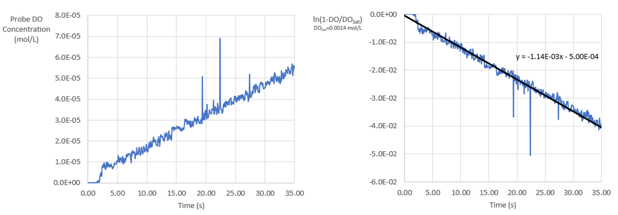
Extracting the volumetric mass transfer coefficient from the probe

In klaLabel4, we present the spatial variation in the dissolved oxygen concentration across the vessel. At early times like this, the dissolved oxygen concentration is not uniform across the tank; the oxygen transfer rate to the fluid is higher than the oxygen advection rate within the fluid (e.g. a large Damkohler number). At long times, as the oxygen saturates the fluid and the mass transfer rate decreases, the dissolved oxygen concentration homogenizes.

Observe that, in this system, most oxygen transport from the bubbles to the liquid occurs in the immediate vicinity of the sparge. Although advection blends this oxygen-infused water through out the system, most of the direct oxygen transfer occurs in this small volume below the impeller.

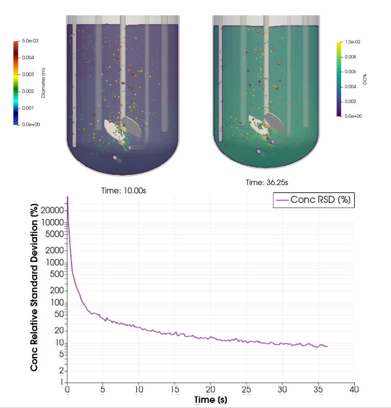
Spatial distribution of dissolved oxygen in the system

In klaLabel5, we show the rate of mass transfer from each bubble to the surrounding fluid. This value is not uniform, as each bubble has a unique surface area, local mass transfer coefficient, and driving concentration different. This behavior leads to differences in mass transfer utility of each bubble. For example, at this snapshot, about 20% of the bubbles are responsible for 80% of the overall mass transfer.

The total mass transfer rate and total mass transfer coefficient for all the bubbles are also calculated automatically by M-Star CFD. As to be expected from the conservation of mass, the transfer rate calculated internally here by M-Star CFD is consistent with the transfer rate extracted from the time-evolution of the oxygen concentration at the probe. This data comes directly from the particles.txt output file.

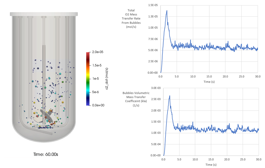
Mass transfer rate computed for the bubble set

A subtle but interesting point is worth addressing: as mass transfer occurs only at bubbles, \(k_L A\) is not a continuous property defined at all points inside the fluid. Indeed, if a certain volume of the fluid contains no bubbles, \(k_L A\) will necessary be zero within that volume. This condition does not imply that oxygen will not exist in a fluid volume that contains no bubbles; the effects of advection and diffusion will push oxygen through the vessel even into regions where there is no direct transfer from the gas bubbles. It is observed in both experiment and simulation that the time evolution of the oxygen concentration at a given point reveals a local timescale associated with oxygen accumulation. This time-constant is indeed continuous across the entire fluid domain and, for well-stirred systems, reclassifying this time-constant as an effective, tank-averaged \(k_L a\) is appropriate. But, in mechanistic sense, the local timescale associated with oxygen accumulation is not necessary equal to the local oxygen transfer rate from the bubbles. The former is property of the (continuous) fluid, while the later is a property of the (discrete) bubbles.

We can further cross-check this output by comparing the system-level mass transfer rate to the system-average concentration differences. From the conservation of species:

\[\dot{C}_f= \frac{k_l A}{V}\left( SC_g-C_f \right)\]

where \(\dot{C}_{f}\) is the time rate of change of the mean dissolved oxygen concentration in the vessel and \(C_g\) is the mean oxygen concentration in the bubbles. At early times, when the concentration of oxygen in the fluid is orders-or-magnitude below the solubility limit, this expression is approximated as:

\[\dot{C}_f \approx k_l a SC_g,\]

In klaLabel6, we present the time-evolution of \(\dot{C}_f\), a value reported directly by the solver in the scalar_o2.txt output file. At steady state, the fluid is accumulating oxygen at a rate of 1.5x10^-6 mol/L/s. This rate is consistent with the time-evoltuion of the concentration at the probe location. As discussed above, the saturated oxygen concentration for this system (\(SC_g\)) is equal to 0.0014 mol/L. These values suggest a \(k_L a\) value of about 4 1/hr, which is consistent with that reported above using a more rigorous analysis. Note that this simplified approach assumes that the tank is well-stirred and the dissolved oxygen concentration is very low compared to the saturated limit.

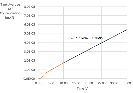
Validating \(k_L a\) using the mean oxygen concentration of oxygen in the vessel

Finally, we can perform a complete oxygen mass balance from the perspective of the bubbles. In klaLabel7, we present the time-evolution of the oxygen mass flux (i) entering the system as bubbles through the sparge, (ii) leaving the system as bubbles through the free surface, and (iii) leaving the bubbles via mass transfer to the liquid. This data comes directly from the particles_bubbles.txt output file. As expected, the bubbles entering the system are injecting more oxygen than the bubbles are taking from the system as the exit the free surface. The difference between these values is equal to the mass transfer to the fluid. Note that, as expected from the conservation of species, this difference is consistent with total mass transfer rate in to the liquid and the increase in oxygen concentration in the fluid.

In this sense, we have a complete bookkeeping of all oxygen in the system from the perspective of both the gas and the liquid phases.

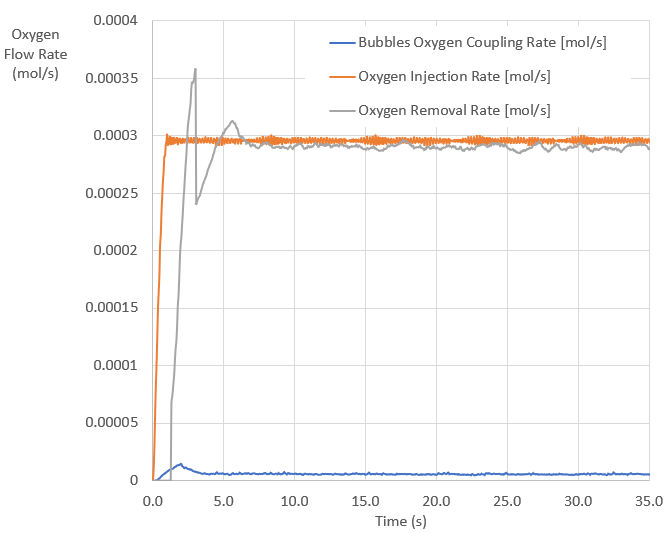
Bookkeeping of each gas species entering/leaving the system through the bubbles

Investigating the Effects of Break-up

Bubble breakup in turbulent fluids is caused by dynamic forces on the bubble, which are a function of the fluid density and local fluid energy dissipation rate. [2] If this local turbulent energy exceeds the stabilizing surface energy due to surface tension, a break-up event is expected. From an energy balance, the equilibrium bubble diameter \(D_e\) can be approximated as:

\[D_e \approx \frac{ \sigma^{\frac{3}{5}}}{ \rho^{\frac{3}{5}} \epsilon^{\frac{2}{5}}}\]

where \(\sigma\) is the bubble/liquid surface tension and \(\rho\) is the fluid density. A break-up event is expected when a bubble enters a region wherein the local equilibrium bubble diameter defined by this equation is smaller than the current bubble diameter. In most cases, bubble undergo binary break-up processes into two satellite bubbles. [8] The volume fraction distribution function of these two satellites tends to be U-shaped and centered at 0.5, such that break-up in to equal diameter satellites has the lowest probability. [9-10]

The break-up implementation in M-Star CFD(R) follows this mechanistic approach presented above, wherein the user defines (i) if a bubble realizes a break-up event and (ii) the volume fraction of the first satellite generated by this break-up event. A sample code is presented in klaLabel8:

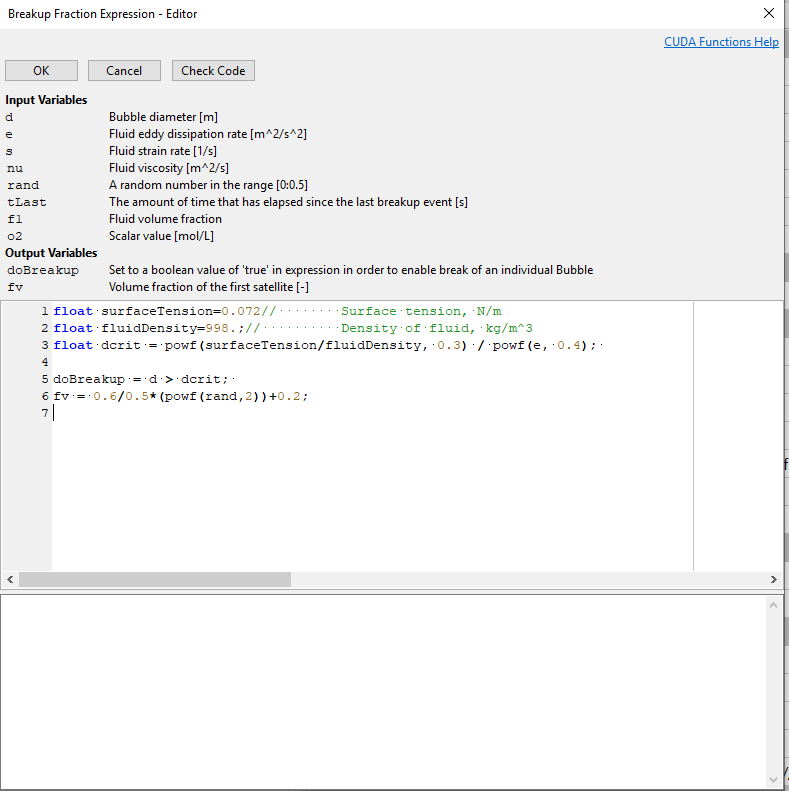
V-shaped daughter size break-up model

The doBreakup conditional expression initiates a break-up is consistent with the equilibrium bubble diameter defined above. In this example, the daughter volume fraction expression is designed to mimic the U-shape distribution defined by the literature.

In klaLabel9, we present the time-evolution of the overall mass transfer coefficient, as automatically calculated and reported for the bubbles for systems with bubble break-up enabled. This data comes directly from the particles_bubbles.txt output file. In addition to the U-shaped break-up, random break-up fv=rand and equal daughter size break-up fv=0.5 were also considered. Including bubble break-up into the model increased the predicted overall mass transfer coefficient by about 10%, a behavior which improved the model predictions relative to experiment. Differences between the various break-up kernels were small, suggesting that the ability to break-up (in this system) is more important than the exact shape of the distribution function.

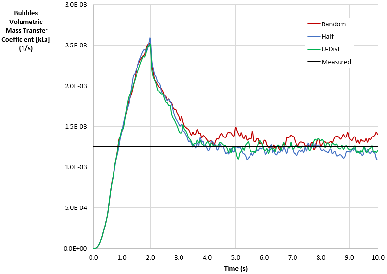
Effects of break-up kernel on volumetric mass transfer rate

To understand the physics driving this outcome, in klaLabel10 we present a snapshot of the energy dissipation rate within the tank, along with the functional form of the equilibrium bubble size for an air-water system. Note that the highest predicted energy dissipation rates predicted from the solver are on the order of 10 m²/s³, which occur immediately behind the impeller. The expected equilibrium bubble size in this region is expected to be around 1.3 mm. Since bubbles enter the system at 1.1 mm, the effects of break-up are not expected to be pronounced in the immediate vicinity of the impeller. Therefore, since most of the overall mass transfer occurs in this region due to the high local energy dissipation rate, activating bubble break-up is not expected to have an order-of-magnitude effect on the predicted mass transfer rate.

Further from the impeller, the energy dissipation rate is around 1 m²/s³, which corresponds to an equilibrium bubble size around 3-4 mm. Larger bubbles, which form above the impeller via repeated coalescence events, will therefore break-up into smaller satellites. This break-up will increase the mass transfer area above the impeller, leading to a modest increase in the overall mass transfer rate.

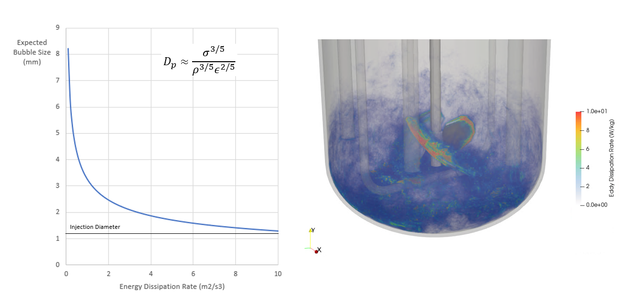
Predicted bubble size as a function of energy dissipation rate

These effects can be further quantified by investigating the bubble size distribution, as shown in klaLabel11. As expected, allowing for break-up shifted this distribution to smaller bubble diameters. For systems with break-up, bubbles smaller than the 0.11 mm bubbles entering through the sparge are realized. This shift also informs the mean bubble diameter (shown in the legend). The net effect of these smaller bubbles is an increased surface area that enables additional mass transfer.

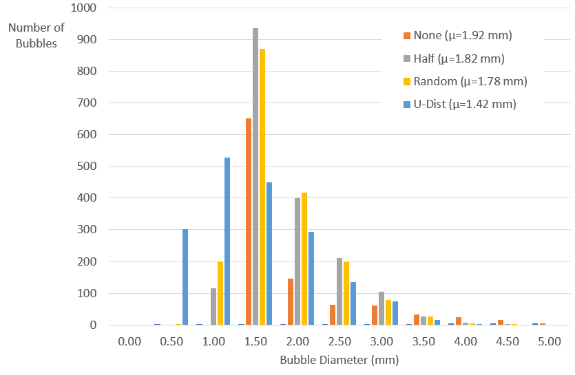
Bubble size distribution as a function of break-up model

Effects of Impeller Speed and Gas Flow rate

In klaLabel11, we compare the predicted overall mass transfer coefficient to the measured values at various impeller speeds and flow rates. These models used the same bubble and species transport mechanics described above. The only changes between models were the gas flow rate and impeller speed. The predicted overall mass transfer coefficient reported came directly from the particles_bubbles.txt output file associated with each run. The predictions agree with experiment in both magnitude and trend: higher impeller speed and higher gas flow rate lead to higher mass transfer rates. Higher impeller speeds lead to larger energy dissipation rates that, as discussed above, increase both \(k_L\) and the bubble break-up events. Higher gas flow rates, in addition to increasing the energy dissipation rate, increase the mass transfer surface area. The agreement across the range of operating conditions sampled here suggest that the solver is correct.

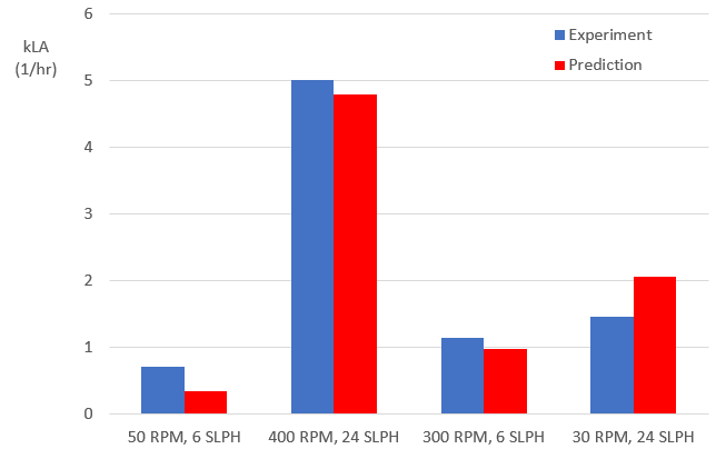
Bubble size distribution as a function of break-up model

Modeling Oxygen Consumption and Carbon Dioxide Scrubbing

In addition to modeling oxygen transfer, species reaction and CO₂ scrubbing are straightforward to implement in the model. In this next iteration, we add biomass to the system which consumes dissolved oxygen while producing carbon dioxide. The O₂ consumption and CO₂ production are modeled as follows:

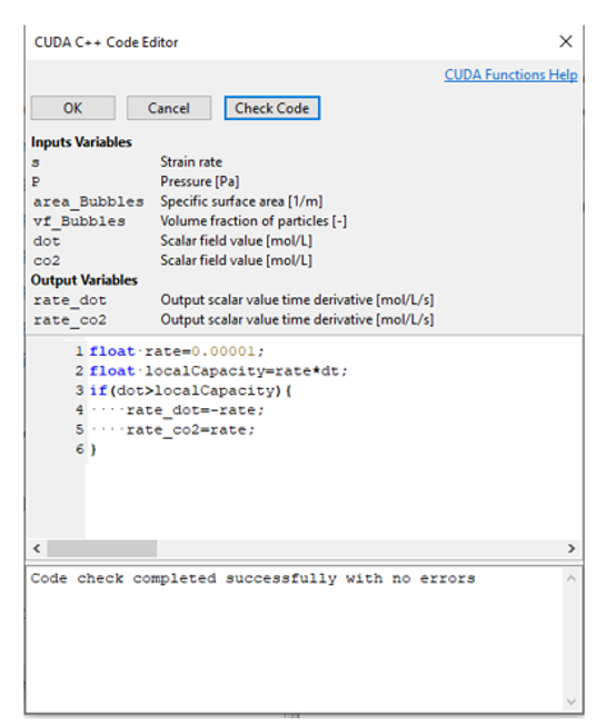
Biomass reaction kinetics for O₂ consumption and CO₂ production

This reaction is simple: CO₂ is produced at a rate equal to O₂ consumption. More sophisticated models would couple these two rates, a functionally that can be included in the model as needed. Bubbles enter the system as pure oxygen, per the injection characteristics specified above. The background concentration of both CO₂ and O₂ are taken the be 0 mol/L. The solubility of CO₂ is taken to be 0.83. [7]

With these reactions present, the dissolved oxygen concentration in the liquid will not converge to the saturation limit. Rather, the concentration will approach some steady state value that represents a balance between oxygen transfer from the bubbles and oxygen consumption by the biomass. Likewise, the carbon dioxide concentration is expected to increase until the rate of transfer to the bubbles is equal to the rate of production due to the reaction.

In klaLabel11k, we present the time-evolution of the dissolved oxygen and carbon dioxide concentrations, along with the transfer and consumption/production rates. This data comes directly from the scalar_o2.txt and scalar_co2.txt output files. The immediate convergence of the oxygen concentration to a near-zero value indicates that the reaction is oxygen limited. This result is unsurprising, given the high (and constant) oxygen consumption rate (\(10^{-5}\) mol/L/s) relative to the low gas/liquid oxygen mass transfer rate (\(\approx 10^{-6}\) mol/L/s, see klaLabel5)

Conversely, the carbon dioxide concentration increases slowly (relative to the dissolved oxygen concentration) to a much higher steady state value. This effect is also a consequence of the low mass transfer coefficient between the bubbles and the surrounding fluid; high dissolved carbon dioxide concentrations are required to drive mass transfer into the bubbles at a rate that matches production by the biomass. Eventually, the CO₂ concentration increases to the point wherein the mass transfer to the bubbles equilibrates with the CO₂ production by the reaction. When this point is reached, the CO₂ concentration equilibrates.

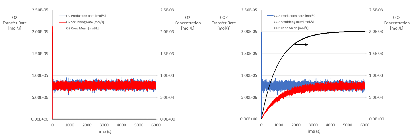
Time-evolution of gas transfer and production rates.

We can also examine the species balance from the perspective of the bubbles. In klaLabel12, we show the time-evolution of the mass flux (mol/s) of each species due to bubbles entering/leaving the system. This data comes directly from the particles.txt output file. Due to exchange with the fluid, the oxygen content of the bubbles is decreasing; more oxygen enters through the bubbles coming out of the sparge than leaves through the bubbles exiting the tank. The difference is equal to the oxygen transfer rate to the fluid. Likewise, the carbon dioxide content of the bubbles increases; more carbon dioxide leaves through the bubbles exiting the tank and comes in through the sparge (which is zero). The difference is equal to the carbon dioxide transfer rate from fluid. In the system without reactions, the oxygen bubbles remained pure oxygen. Although the volume of each bubble decreased due to mass transfer, the oxygen concentration was constant. In this system, carbon dioxide transfer from the fluid to the bubbles cause the bubble composition to evolve over time. This change in concentration, which is automatically handed in the code, will inform the mass transfer rates of each species as the bubble rises.

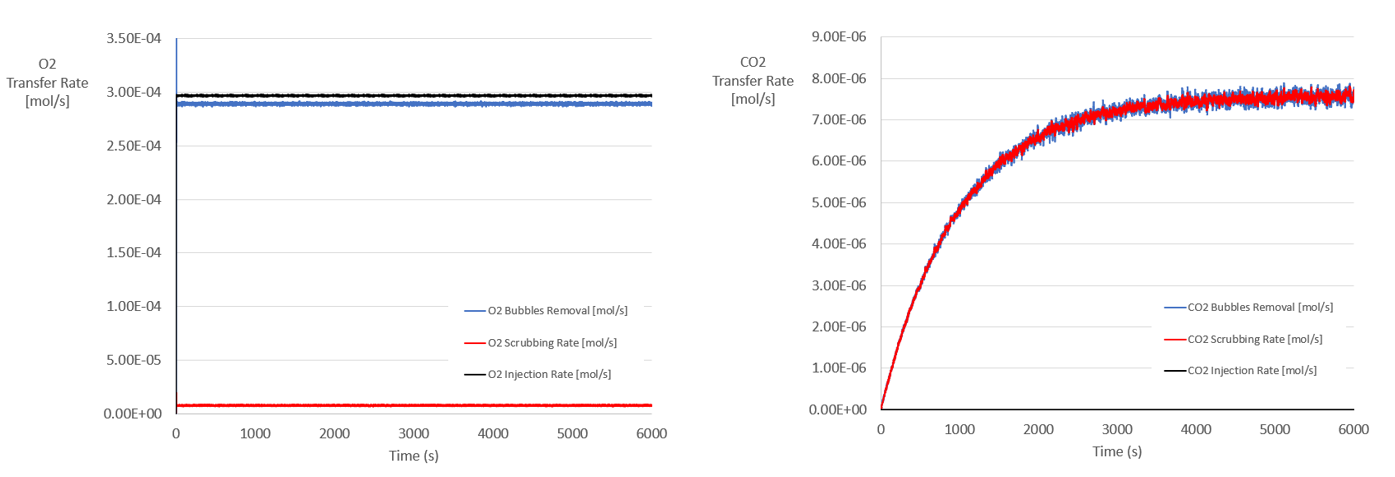
Time-evolution of mass flux and concentration of each species

In klaLabel13, we present a snapshot of the carbon dioxide composition within each bubble during steady state conditions. Since bubble enter the system as pure oxygen, their initial carbon dioxide concentration is zero. At equilibrium conditions, however, the carbon dioxide concentrations of the bubbles leaving the surface evolves to a few percent. This information can be used to predict headspace gas compositions.

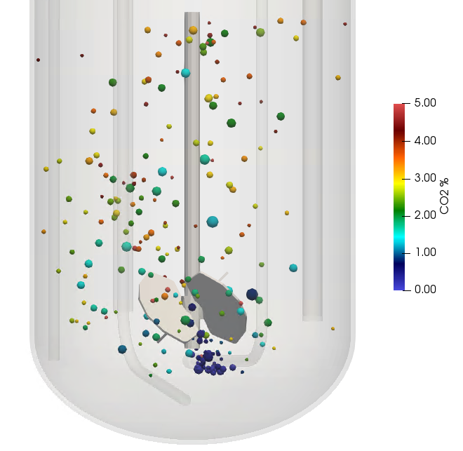
Instantaneous percent concentration of carbon dioxide in each bubble

In this sense, again, we have a complete bookkeeping of each species in the system from the perspective of both the gas and the liquid phases.

Summary

In this module, we examined the physics driving mass transfer between bubbles and a fluid. In addition to oxygen transport, we examine the effects of reactions and gas bubble scrubbing.

References

[1] Calderbank, P.H and Moo-Young, M.B., 1961. The continuous phase heat and mass-transfer properties of dispersions. Chem. Ens. Sci., 16, 39-54.

[2] Kawase, Y. and Moo-Young, M.B., 1990. Mathematical Models for Design of Bioreactors: Applications of Kolmogoroff’s Theory of Isotropic Turbulence, Chem. Eng., 43, 819-841

[3] Pope, S. B., 2000. Turbulent Flows. Cambridge University Press, Cambridge

[4] Yang, H., et al., General formulas for drag coefficient and settling velocity of sphere based on theoretical law

[3] Brown, P.P. and Lawler, D.F., 2003. Sphere Drag and Settling Velocity Revisited. J. Environ. Chem. Eng. 129, 222-231.

[5] Boshenyatov, B., 2012. Laws of Bubble Coalescence and their Modeling. New Developments in Hydrodynamics Research 08, 211-240.

[6] Geary, N. W., & Rice, R. G., 1991. Bubble size prediction for rigid and flexible spargers. A.I.Ch.E. Journal,37,161.

[7] Sander, R., 2015. Compilation of Henry’s law constants for water as solvent, Atmos. Chem. Phys., 15, 4399–4981

[8] Krakau, F. and Kraume, M., 2019. 3‐D Observation of Single Air Bubble Breakup in a Stirred Tank. Chemical Engineering & Technology. 42, 1357-1370

[9] Xing, C.; Wang, T.; Guo, K.; Wang, J., 2015. A Unified Theoretical Model for Breakup of Bubbles and Droplets in Turbulent Flows. AIChE J.,61, 1391.

[10] Sungkorn, R., Derksen, J.J., Khinast, J.G., 2012. Euler–Lagrange modeling of a gas–liquid stirred reactor with consideration of bubble breakage and coalescence. AIChE J. 58, 1356–1370.