Initial Size Distribution
Applicability


Distribution Type
These are the options for initial particle size distribution. All particle types are described using the same distribution types.
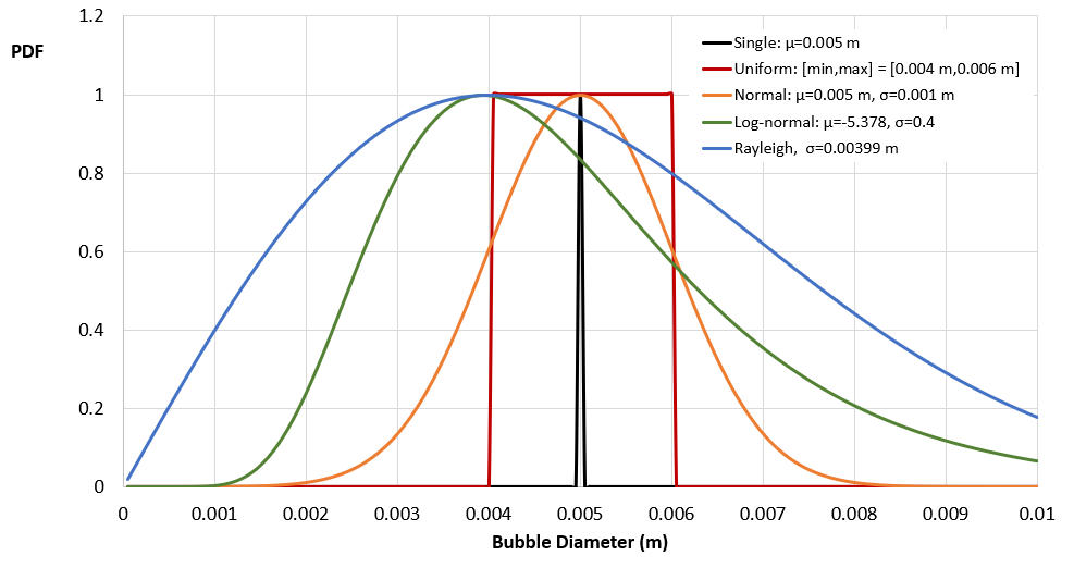
A comparison between the five continuous probability density functions is shown below. Note that each of these distributions, with the parameters specified in the legend, generates a mean particle diameter of 0.005 m.
Single
The diameter of the particles is set by the user and assigned to all particles. This condition represents the addition of monodispersed particles.
- Diameter
default length scale | User-defined diameter. Default is set to 0.001 m. Users can enter their own value.
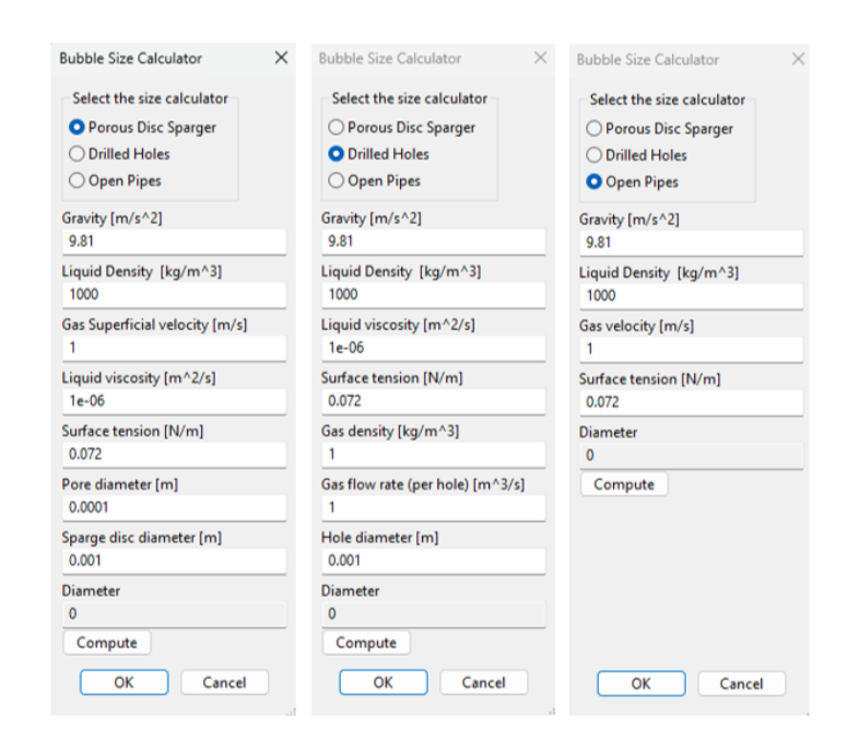
If the selected particle is a Gas Bubble, the
 icon appears, which opens a Bubble Size Calculator. Within this calculator, three sparge types are available: Porous Disc Sparger, Drilled Holes, and Open Pipes. Pressing the Compute button evaluates the diameter based off the user-defined input parameters.
For each sparge type, the calculator uses literature correlations to predict the initial bubble size as a function of the fluid properties and flow conditions. For the Porous Disc Sparger, the initial bubble size is calculated from the correlation developed by Kazakis et al. For the Drilled Holes and Open Pipe correlations, the initial bubble size is calculated from the correlations presented by Geary and Rice. Within this work, Equations 19–20 are used for Drilled Holes. Equation 30 is used for open pipes.
Uniform
The diameter of each particle is randomly sampled at runtime from a uniform probability density function with a user-set minimum and maximum diameter, such that:
\(p(d)=\begin{cases}{\frac {1}{\textrm{max}-\textrm{min}}}&{\text{for }}d\in [\textrm{min},\textrm{max}]\\0&{\text{otherwise}}\end{cases}\),
where the mean particle diameter is defined by: \(d_m=\tfrac{1}{2}(\textrm{max}+\textrm{min})\).
- Diameter Minimum
default length scale | User-defined minimum particle diameter. Default is set to 0.001 m.
- Diameter Max
default length scale | User-defined minimum particle diameter. Default is set to 0.002 m.
Normal
The diameter of each particle is randomly sampled at runtime from a normal probability density function with a user-set mean and standard deviation: \(\mu\) and \(\sigma\), such that:
\(p(d)=\displaystyle {\frac {1}{\sigma {\sqrt {2\pi }}}}e^{-{\frac {1}{2}}\left({\frac {d-\mu }{\sigma }}\right)^{2}}\),
where the mean particle size is defined by \(\mu\).
- Diameter Mean
default length scale | The mean value of the probability density function. Default is set to 0.001 m.
- Diameter Standard Deviation
default length scale | The variance of the probability density function. Default is set to 0.001 m.
Log Normal
The diameter of each particle is randomly sampled at runtime from a log-normal probability density function with a user-set log mean and log standard deviation: \(\mu\) and \(\sigma\), such that:
\(p(d)=\displaystyle {\frac {1}{d\sigma {\sqrt {2\pi }}}}\ \exp \left(-{\frac {\left(\ln d-\mu \right)^{2}}{2\sigma ^{2}}}\right),\)
where the mean particle size is defined by, \(d_m=\displaystyle \exp \left(\mu +{\frac {\sigma ^{2}}{2}}\right).\)
- Mean Log Diameter
unitless | The expected value of the natural logarithm of the particle diameter. Default value is set to -6.928. The mean log diameter is a dimensionless quantity defined using a reference length scale. We set this reference length scale to 1 m, regardless of the Unit Settings.
- Standard Deviation Log Diameter
unitless | The standard deviation of the natural logarithm of the particle diameter. Default value is set to 0.2. The standard deviation of the log diameter is a dimensionless quantity defined using a reference length scale. We set this reference length scale to 1 m, regardless of the Unit Settings.
- Particle Diameter Mean
m | We present for reference the dimensionalized mean particle diameter, as computed from the mean log diameter and the standard deviation of the log diameter. This parameter is dimensionalized using a reference length scale of 1 m, regardless of the Unit Settings.
- Particle Diameter Standard Deviation
m | We present for reference the dimensionalized particle standard deviation, as computed from the mean log diameter and the standard deviation of the log diameter. This parameter is dimensionalized using a reference length scale of 1 m, regardless of the Unit Settings.
Note
More information about the dimensionless nature of the log-normal parameters is available here.
Rayleigh
The diameter of each particle is randomly sampled at runtime from a Rayleigh probability density function with a user-set scale parameter, such that:
\(p(d)= \frac{d}{ \sigma ^{2} }e^{-d^{2}/\left(2\sigma^{2}\right)},\) where the mean particle size is defined by:
\(d_m=\sigma {\sqrt {\frac {\pi }{2}}}.\)
- Distribution Scale Parameter
default length scale | The scale parameter of the Rayleigh distribution, which is also equal to the distribution mode. The default value is set to 0.001 m.
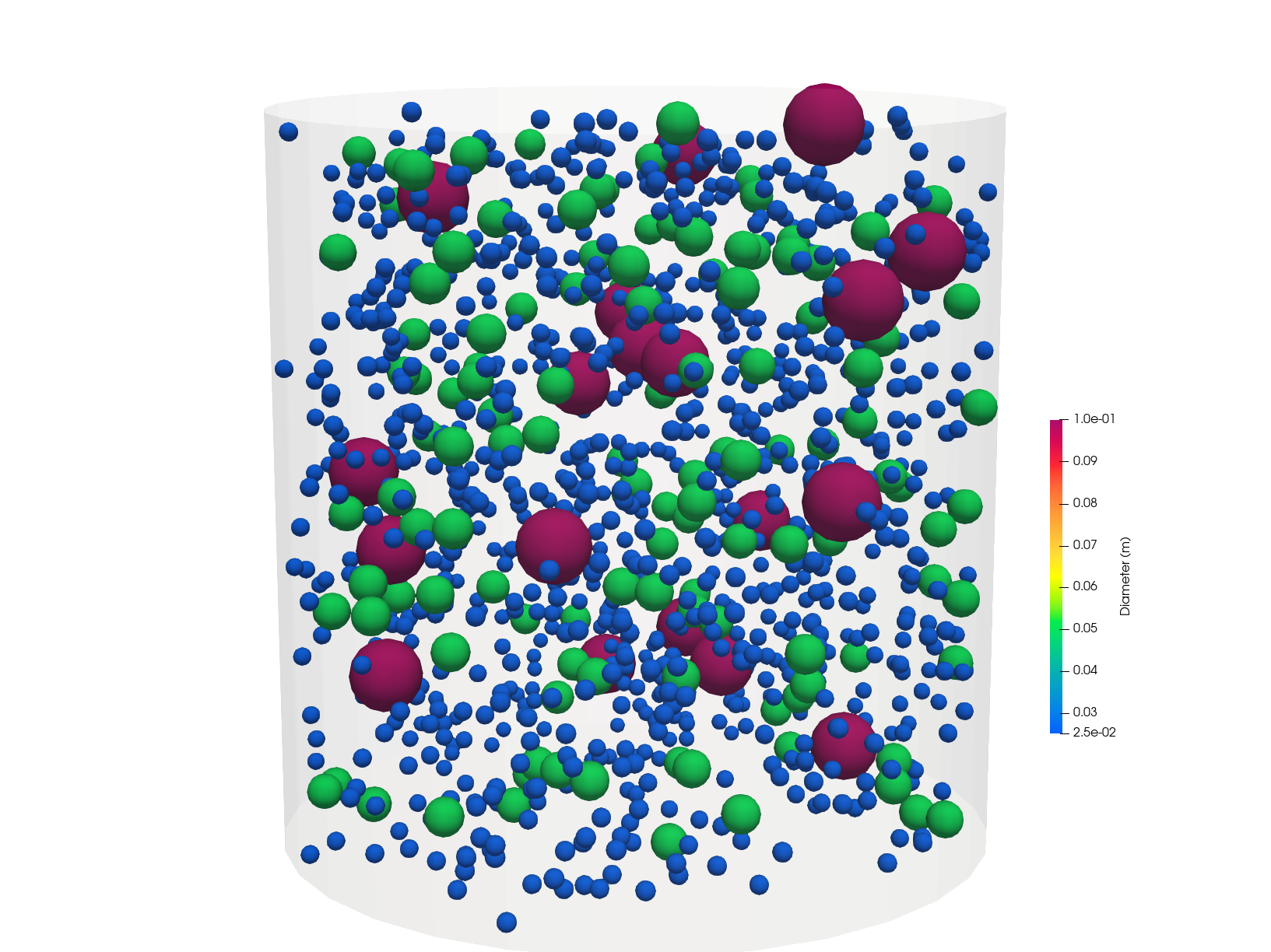
Discrete Diameter Distribution
This option defines a custom initial particle diameter distribution. The distribution is specified as a table that pairs specific particle diameters with their corresponding probabilities, effectively forming a particle size distribution. While the sum of the probability values must equal unity, the shape of the distribution can be arbitrary.
- Diameter Distribution Table
This table represents the initial diameter distribution of particles added to the system. It is a normalized histogram representing the distribution of particle diameters.
The table consists of two equal-length columns: (i) particle diameter and (ii) probability.
The unit on values in the diameter column is the model base unit (meters by default). The probability column is unitless.
The particle diameter specifies the initial diameter of the particle introduced into the system. The probability determines the likelihood of injecting a particle with the corresponding diameter. This distribution is randomly sampled at runtime when adding particles to the system.
The table must contain at least one row but no more than 50 rows. This is a two-column table.
Download Sample File: Diameter Distribution
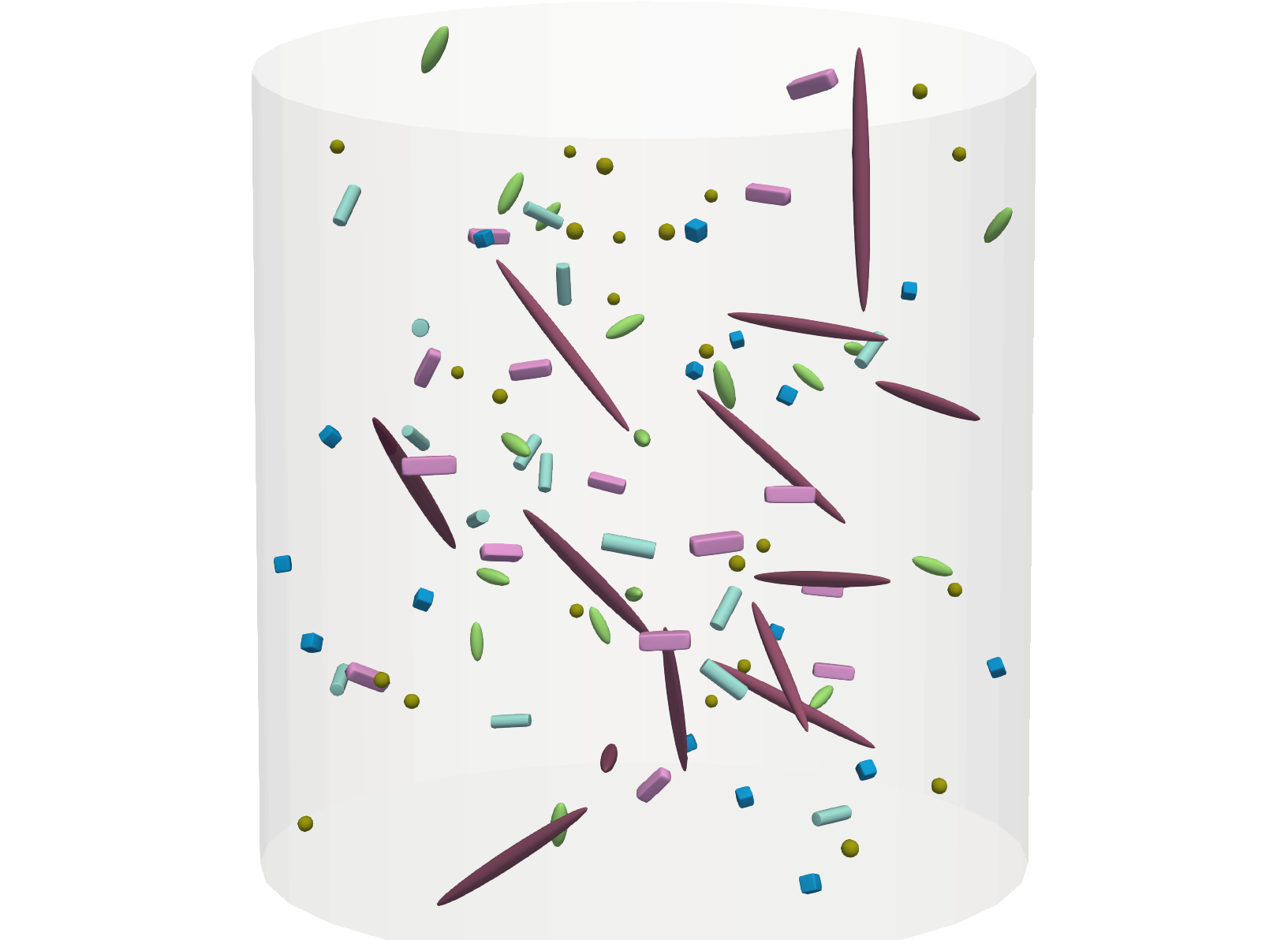
Discrete Superquadric Distribution
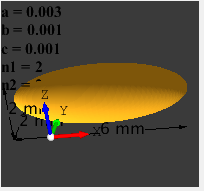
Superquadrics are a family of geometric shapes, including spheres, ellipsoids, cylinders, and cubes. They use shape parameters that control curvature and sharpness. Defined by implicit equations involving exponentiation of coordinates, superquadrics offer a flexible representation for different geometric forms.
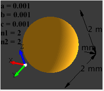
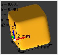
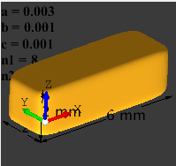
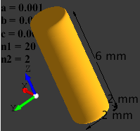
Superquadrics are defined by five parameters: three radii (a, b, c) corresponding to the semi-axes lengths along the x, y, and z directions; and two shape parameters (n1, n2) that control the smoothness or angularity of the shape. The radii determine the overall dimensions of the superquadric, while the shape parameters adjust the curvature of the surfaces and the sharpness of the edges. For instance, setting n1 and n2 to values greater than 2 results in shapes with sharper edges, such as cubes or cuboids, whereas values equal to 2 produce smoother shapes like spheres or ellipsoids.
The table below demonstrates some common example shapes generated by tuning the radii and shape parameter.
Shape |
a |
b |
c |
n1 |
n2 |
Preview |
|---|---|---|---|---|---|---|
Sphere |
1 |
1 |
1 |
2 |
2 |
|
Ellipsoid (Pill) |
3 |
1 |
1 |
2 |
2 |
|
Long Ellipsoid (Needle) |
1 |
1 |
15 |
2 |
2 |

|
Cube |
1 |
1 |
1 |
8 |
8 |
|
Cuboid |
3 |
1 |
1 |
8 |
8 |
|
Cylinder |
1 |
1 |
3 |
20 |
2 |
|
This injection option defines a custom initial superquadratic shape distribution. The distribution is specified as a six-column table that pairs specific particle shapes (represented using the five superquadratic shape parameters) with their corresponding probabilities. These data effectively form a particle shape and size distribution. While the sum of the probability values must equal unity, the shape of the distribution can be arbitrary.
- Superquadric Distribution Table
This table represents the initial shape/size distribution of particles added to the system. It is a normalized histogram representing the distribution of particle shapes/sizes, as represented using the five superquadratic shape parameters.
The table consists of six equal-length columns. Columns 1–3 represent the three radii of the superquadratic. Columns 4–5 represent the two shape parameters. Column 6 represents the probability.
Columns 1–5 define the shape/size of the particle introduced into the system. The probability determines the likelihood of injecting a particle with the corresponding shape/size. This distribution is randomly sampled at runtime when adding particles to the system.
The table must contain at least one row but no more than 50 rows. This is a multi-column table.
Download Sample File: Superquadric Distribution
Discrete Volume Distribution
This option defines a custom initial particle volume distribution. The distribution is specified as a table that pairs specific particle diameters with their corresponding volume fractions, effectively forming a particle volume distribution. While the sum of the volume fractions must equal unity, the shape of the distribution can be arbitrary.
- Volume Distribution Table
This table represents the initial volume distribution of particles added to the system. It is a normalized histogram representing the distribution of particle volume.
The table consists of two equal-length columns: (i) particle diameter and (ii) volume fraction.
The units on the diameter column are the model base unit (meters by default). The volume fraction column lists the percentage.
The particle diameter specifies the initial diameter of the particle introduced into the system. The volume fraction determines the fraction of the total injected particle volume that corresponds to this diameter. This distribution is randomly sampled at runtime when adding particles to the system.
The table must contain at least one row but no more than 50 rows. This is a two-column table.
Download Sample File: Volume Distribution
Initial Diameter UDF
The diameter of each particle added to the system is randomly sampled at runtime from a user-specified particle diameter probability mass function. Although the sum of the mass function must sum to unity, this shape of the distribution can be arbitrary.
The custom diameter distribution is a number histogram—it describes the total number of particles within each user-defined bin.
- Initial Diameter UDF
m | This UDF defines the initial diameters of the particles entering the system. This is a System UDF.
Download Sample File:
Initial Diameter UDF
Important
Both of these custom distributions define a particle-size histogram grouped by a set of user-defined particle diameter bins. This distribution is randomly sampled at runtime when adding a new particle to the system. The outcome of this random sampling determines the particle diameter.