Using Custom Particle Variables to Track Particle Exposure
Overview
This guide demonstrates how to use Custom Particle Variables and Global Variables to track particle exposure to local fluid conditions. From stem cells to sand slurries, particles are used to simulate different phenomena across a range of engineering disciplines. With M-Star, we can configure custom particle variables to capture hydrodynamic conditions and gain valuable insight into the particles exposure to local fluid conditions. Using custom variables, we can “equip” each particle with a custom camera that records the conditions it experiences through time. These conditions can then be analyzed to gain insight into the problem at hand.
Model Setup
Let’s set up an example that highlights the custom particle variables and some global variables that we can derive from them.
We’ll start with a simple geometry:
Create a Static Body and add a Cylindrical Tank. Select Flat for End 1 (bottom of the tank).
Create a Moving Body and add a Rushton. Change the Diameter of the Rushton to 0.33 m and the Rotation Speed of the Moving Body to 100 RPM.
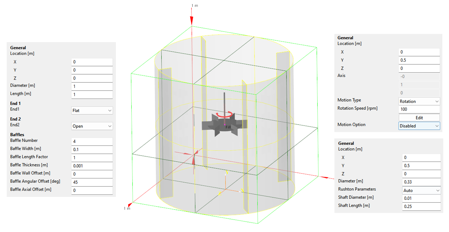
We can also change the resolution to NX = 150, for example, or more depending on your hardware.
Particle Setup
Now let’s add some particles:
Create Particles – Tracers and select a Cuboid as the geometry.
Change the number of dumped particles to 1.000.000 and the Location of the Cuboid to [0.2, 0.65, 0].
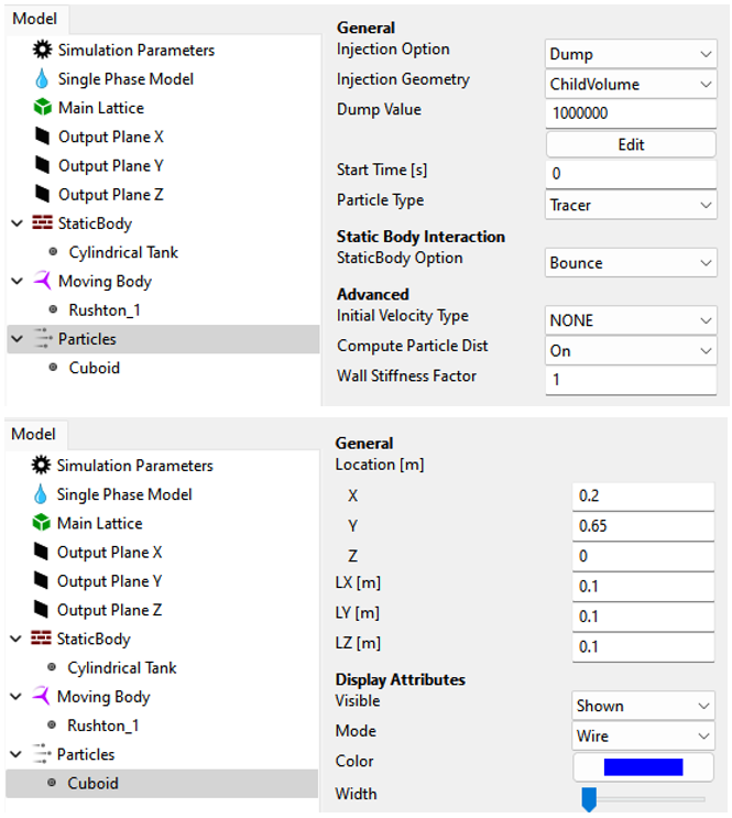
Note that we are using Tracer Particles for simplicity, but we may use any other particle type, such as DEM particles.
Define Stress Criterion
First add a Custom Fluid Variable before we configure our particles. This Custom Fluid Variable serves as the distinction between ‘stressed’ and ‘unstressed’ conditions for the particles. This could be the Energy Dissipation Rate (EDR) as an indicator of hydrodynamic stress, a specific scalar concentration, or any other local fluid condition defined in your User-Defined Function (UDF).
For the following example, we’ll use the EDR:
Create a Custom Variable or Fluid Variable (depending on your M-Star Version) and rename it to ‘stressful’.
Add your expression and choose your threshold. We consider a Fluid Voxel as ‘stressful’ if we exceed a local Energy Dissipation Rate of 1.5 W/m^3.
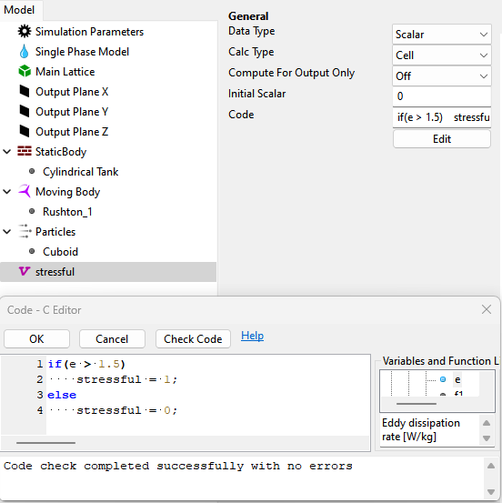
We will use this Custom Fluid Variable to determine our stressed particles.
Custom Particle Variables
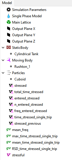
Create a Custom Particle Variable: Select the Particles and Add – Add Custom Variable or Create – Variables - Particle Variable (depending on the M-Star Version you are using).
Rename the Variable to ‘stressed’:
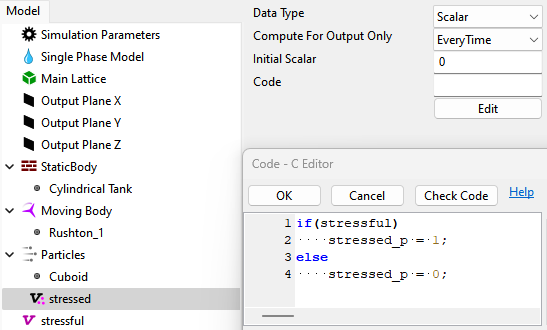
We are now marking the particles as ‘stressed’ if they are in a position of the local fluid that is considered ‘stressful’. We can use this for visualization in M-Star Post or Paraview:
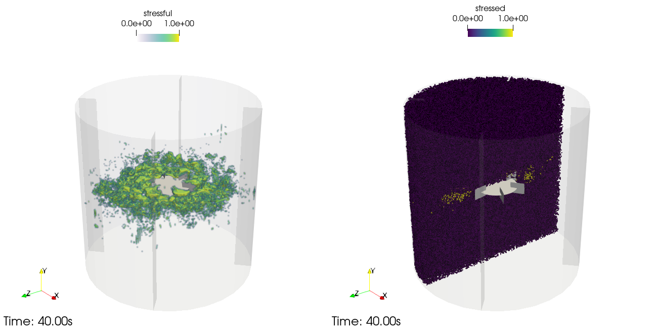
Left: Stressful condition in the liquid. Right: Stressed particles.
This is the basis of our analysis. We can extend this further to record the time that particles spend in high stress regions and the frequencies at which they experience these conditions. We will start by recording the total amount of time that a particle is in the ‘stressed’ state.
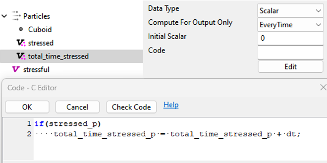
Add another Custom Particle Variable and rename it to ‘total_time_stressed’. Add the timestep dt at each timestep to get the total time inside stressed regions.
In order to check if a particle has reached or left a stressed zone, we need to know our current particle state as well as the state from the previous timestep. This works very much like a loop.
It’s now important to introduce a key concept in the M-Star GUI: the order of the Custom Variables in the GUI is the order of operations in the solver. A variable higher on the hierarchy will be informed before the particle lower on the hierarchy. By introducing another Particle Variable that has the information from the previous timestep, we can check if we just entered or left such a region.
Add another Custom Particle Variable and rename it to ‘stressed_previous’. We will overwrite this value with ‘stressed’ at the end of our algorithm.
Add one more Custom Particle Variable and rename it to ‘entered_stressed’. We will flag particles that have just entered a high stress region during our current timestep by identifying particles that are stressed now and have not been stressed the timestep before:
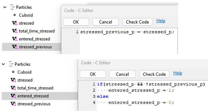
Keep in mind that the order in the GUI tree is important as it defines the order of variable operations. Also make sure that you include the ‘!’ in front of the stressed_previous_p Variable for the ‘entered_stressed_p’ Variable.
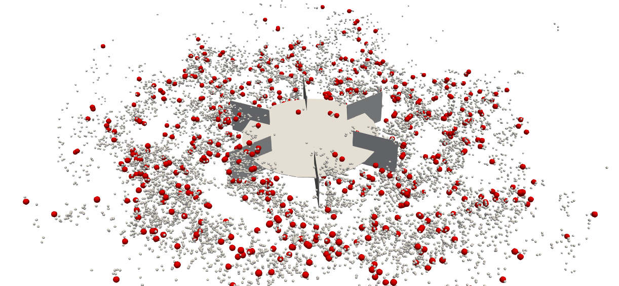
Stressed particles are in gray and particles that have just entered the stressed region are in red.
Now, we want to add a counter that records how often we enter a high stressed region:
- Add another Custom Particle Variable and rename it to ‘n_entered_stressed’. This is just a simple counter:

- Add another Custom Particle Variable and rename it to ‘freq_entered_stressed’. This is a frequency. We divide the counter by the total time:

This is already interesting information, but we also want information about the length of the individual trips through high-stress regions.
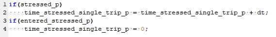
- Add another Custom Particle Variable and rename it to ‘time_stressed_single_trip’. We record the time inside a high stress region but we reset this value each time a particles enters a high-stress region:
Global Variables for Statistical Reduction
Our particles are now equipped with a set of Custom Particle Variables which allows us to record and evaluate the local environmental conditions without any post-processing. We can also add some Global Variables to extract mean values, maxima, and so forth based on these user-defined properties. As examples, we record the mean frequency at which particles enter high-stress regions. We also record the maximum, the mean, and the relative standard deviation of the time that these particles spend in a single trip through a high-stress region:
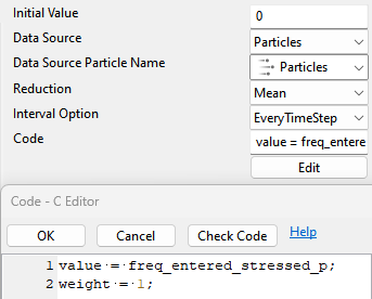
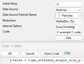
- Add a Global Variable and rename it to ‘mean_freq’. Select the particles as the Data Source, the Mean as the reduction, and the following lines of code:
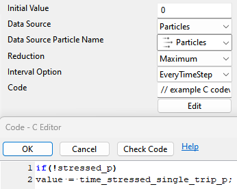
- Add another Global Variable and rename it to ‘max_time_stressed_single_trip’. Here, we exclude the particles that have not finished their trip yet and are still stressed.
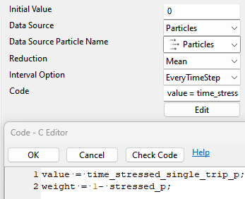
- Add another Global Variable and rename it to ‘mean_time_stressed_single_trip’. We are not considering the ones that are still stressed by the weight for the mean value:
- Add another Global Variable and rename it to ‘RSD_time_stressed_single_trip’. This serves as an indicator if we have a narrow or wide distribution:
We can now run our simulation and look at the results.
Results
We can visualize these user-defined quantities and extract histograms.
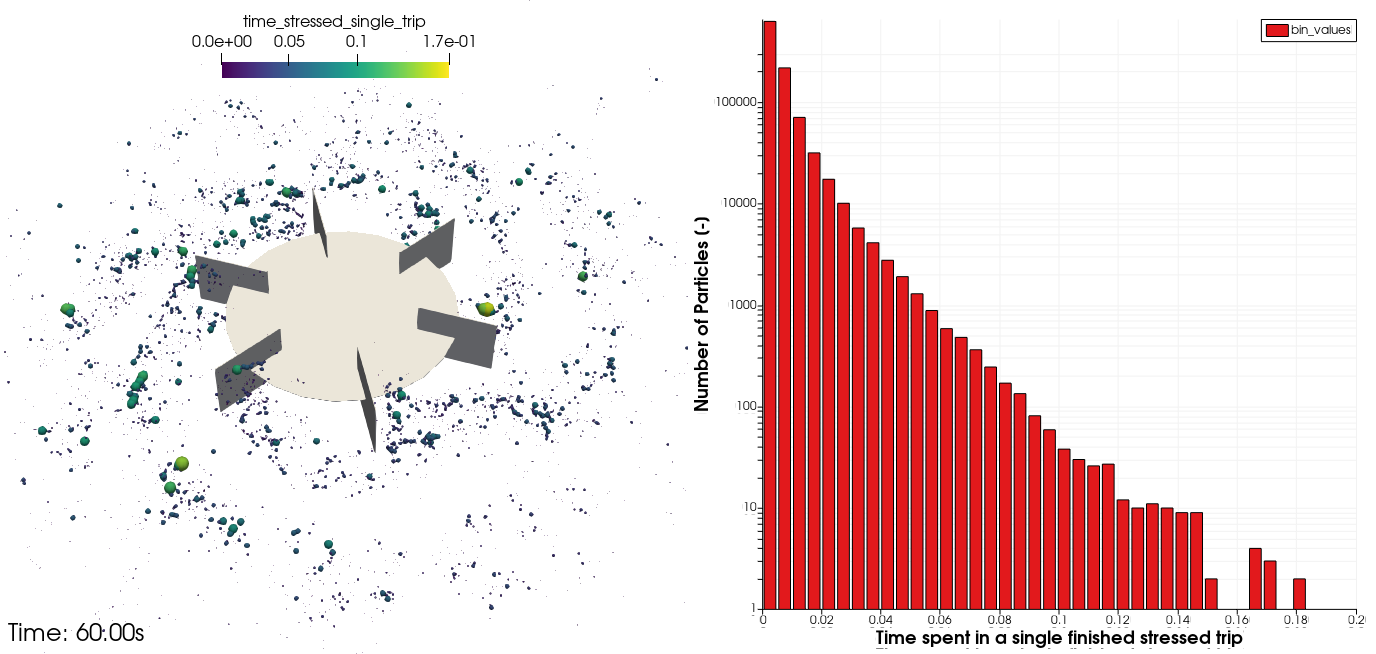
Left: Stressed particles, color, and size indicate the time they have spent in a high stress region.
Right: Histogram of the time that particles spend in a single trip through a high-stress region.
Our Global Variables are used to reduce the analysis to a few scalar values. These can then be used to compare operating conditions and different geometries or scales.
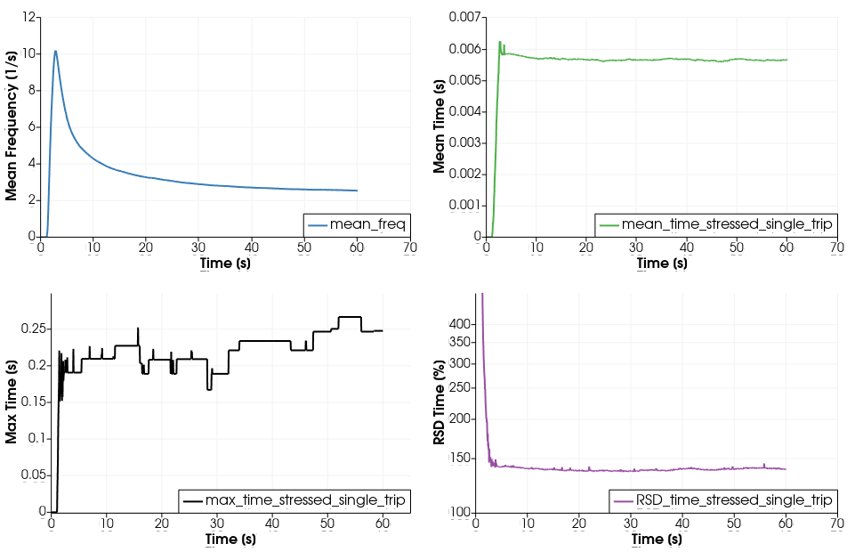
Extracted Global Variables over time
We have now equipped our particles with Custom Variables which can be used to extract single scalar quantities containing highly customized data. The possibilities are essentially endless as a wide variety of phenomena are dependent on local hydrodynamic conditions. The only real disadvantage to this approach is that the user needs to have some idea of the thresholds in advance. Once these are discovered, you can save a lot of time by automatically extracting these statistics when the simulation is performed.