Mixing Bioreactors with Bottom Mounted Impellers

Objective

In this work, we will use M-Star CFD to predict single and multi-fluid blending in tall tanks.

Input Files

Single fluid model.

Multi fluid model.

Conceptual Overview

Most mixing correlations are derived from experiments involving top-entry impellers centered in baffled tanks with a fluid level equal to the tank diameter. While this standard configuration is useful in generating repeatable data sets, it bears little resemblance to the tank and impeller topology present in many pilot and production systems. In most bioreactors, for example, the impeller is off-centered and bottom mounted while the tank is unbaffled and has a fill level that may be several times larger (or smaller) than the tank diameter. These topological differences introduce additional complexities into the flow field, including:

1. dissimilar mixing characteristics across the tank,

2. large spatial variations in the local strain/energy dissipation rates,

3. rigid body swirling/vortexing,

4. density-induced species stratification

These complexities are exacerbated when the vessel is operating in a transitional flow regime, wherein small changes in impeller Reynolds number can lead to large changes in blend time and required operating conditions.

In this work, we use M-Star CFD to predict the single fluid and multi-fluid mixing behavior of bioreactors across a variety of scales, fluid volumes, and impeller speeds. After a review of concepts and definitions, we compare the single-phase blend-time predictions for the Xcellerex XDR 500 and 2000 single-use bioreactors to measured data. Next, we examine a two-fluid mixing problem involving the dilution of a concentrated protein solution. We validate predictions from the two-fluid model to experimental data, then use the model to explore the relationship between density, viscosity and mixing.

Building the Single Fluid Model

The 500 L and 2000 L bioreactor systems, as shown in misc_label5, are geometrically similar. The impellers in both systems are bottom-mounted but off-center, such that the impeller rotation vector is tilted 15 degrees relative to the tank centerline. The vessel diameters are 0.76 and 1.2 m, respectively. The impeller in the 500 L vessel is a three-bladed hydrofoil with a diameter of 0.26 meters. A similar hydrofoil is used in the 2000 L vessel, although it has four blades and a diameter of 0.43 meters.

The simulation resolution was set to 250 lattice points across the tank diameter, a value sufficient to predict a fully-converged power number in both configurations. To assist in blend time prediction, three probes are added to the tank: one near the top surface, one near the center of the fluid volume, and one near the bottom of the vessel.

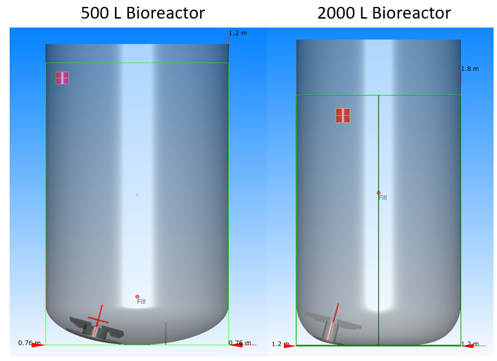
500 L and 2000 L bioreactors used in this investigation. The two systems are geometrically similar. The red cylinder in each system is the dye injection location.

Impeller speeds range from 30 to 200 RPM, depending on operating condition and vessel size. The Courant number was set to 0.05 for all simulations, which ensured that variations in the lattice density remained below 2%. An LES turbulence closure model was applied with the default Smagorinsky coefficient of 0.1.

To assess the effects of surface vortexing, we performed preliminary free-surface simulations of the 500 L bioreactor operating at a 100 L working volume with an impeller speed of 200 RPM. The 200 RPM condition has the largest power per unit volume of any case to be tested, and is expected to generate the most dynamic free surface. For comparison, we also ran the same system with an impeller speed of 30 RPM. The surface tension at the interface was set to 0.072 N/m in both models.

In misc_label5q, we compare snapshots of the free surface from the two operating conditions, taken during steady-state flow conditions. As expected, the free surface velocities for the 200 RPM case are higher than those realized in the 30 RPM case, which presents a flat interface. Although the 200 RPM case presents surface vortexing, the depth of this vortex is still small relative to the fluid height and tank diameter. Even at this maximum power per mass operating condition, the interface is relatively flat and consistent with the interface presented in the 30 RPM case (which has 300x less power per unit volume). Motivated by these observations, we define a flat, free-slip boundary condition at the top surface for all models.

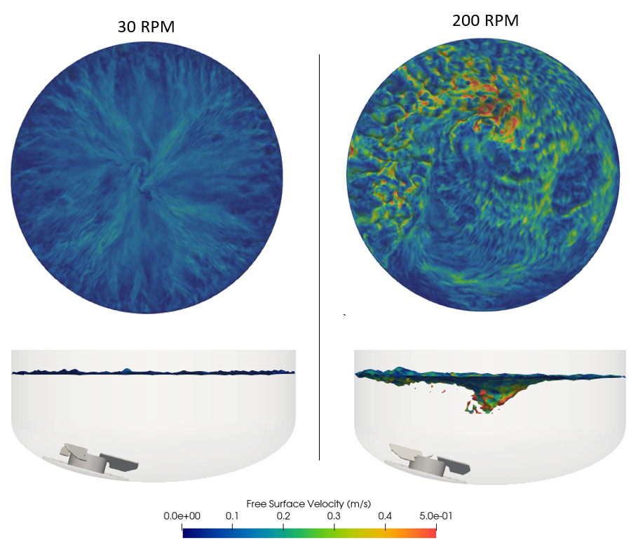
Comparing the effects of impeller speed on free-surface motion and vortexing.

We predict blending by monitoring how a passive dye added just below the top surface homogenizes across the vessel. The initial background concentration of the dye scalar field was set to zero. Then, following a one to two minute start-up and fluid initialization period (depending on impeller speed), the scalar field concentration within the red cylinders shown in misc_label5 was instantaneously set to 1.0. Following this injection, dye transport is governed by the advection/diffusion equation:

\[\frac{d c_j}{dt} = \nabla \cdot D \nabla c_j + \nabla \cdot \left( \vec{v}_j c_j \right),\]

where \(c_j\) is the dye concentration in fluid voxel \(j\), \(D\) is the dye diffusion coefficient, and \(\vec{v}_j\) the fluid velocity vector at voxel \(j\). The dye diffusion coefficient was set to 10^-9 m²/s, a generic value for solute/solvent combinations. Since the effects of diffusion on mass transport are expected to be small relative to advection, the exact value will not strongly influence blending.

We solve the advection portion of the advection/diffusion equation using the (default) Van Leer flux limiter. In addition to providing a second-order accurate solution, the limiter plays an important role in minimizing spurious numerical diffusion. The time-dependent advection/diffusion equation is solved in tandem with the time-dependent Navier-Stokes equations at each time step.

For this closed, non-reactive system, conservation of mass requires that the total number of moles within the system remain constant following the pulse injection. As such, although the local concentration will evolve through time, the global mean concentration (total number of moles divided by total fluid volume) of the dye within the tank is constant.

For these single-fluid blend time simulations, the dye is a passive tracer. That is, the dye concentration does not inform local fluid viscosity and/or density. It is straightforward to link the local and instantaneous scalar field concentrations to the local and instantaneous fluid properties. This functionality will be explored below.

Analyzing the Single Fluid Simulation

In the movie below, we show the time-evolution of the velocity field and concentration field for a 2000 L bioreactor containing 1200 L of water with an impeller speed of 70 RPM. Note that the velocity, turbulence intensity, and local mixing times near the impeller are greater than those near the free surface. The effects of rigid body swirling are apparent in the dynamics of the dye after it first enters the tank. For the first five seconds, the dye just swirls around the top half of the tank. Significant mixing only occurs later as the dye is drawn into the impeller region. This heterogeneous flow behavior is common in tall/unbaffled tanks and has important implications on mixing.

Analyzing the Output

Power Number

In misclabel6, we present the time-evolution of the power number for the 500 L vessel with a 500 L working volume and a 200 RPM impeller speed. We also present the time-evolution of the power number for the 2000 L vessel with a 1200 L working volume and a 115 RPM impeller speed. This data comes directly from the bottomImpeller.txt output files from each simulation. Note that the 500 L vessel impeller power number reaches steady state after about 60 seconds. Prior to reaching this condition, as the impeller is working to accelerate the initially quiescent fluid, the impeller power number is higher than the steady-state value. For the 2000 L vessel, steady state power draw is realized around 90 seconds. This difference is expected, given the larger fluid volume but lower impeller rotational speed in the 2000 L vessel simulated here.

We superimpose on this transient data the reported fully-turbulent steady-state power number for each system, as measured from a torque sensor attached to the shaft. [1,2] At both scales, the predictions are within 10-15% of experiment. Interestingly, although the 500 L vessel has only three blades, the predicted and measured power numbers are higher than those obtained for the four-bladed 2000 L impeller. This behavior is likely due to the position of the impeller relative to the tank bottom. In the 2000 L vessel, the impeller is offset approximately one-half an impeller diameter from the tank wall. In the 500 L vessel, the impeller is immediately adjacent to the wall. This positioning increases the resistance experienced by the impeller in the 500 L vessel, thereby increasing the calculated power number. At these operating conditions, of course, the absolute power requirement for the 2000 L is still higher.

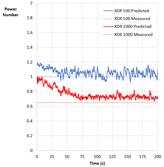
Comparing the predicted to measured power numbers for the XDR 500 and XDR 2000 systems.

Blend time Predictions

In this section, we compare two approaches for tracking blending and homogenization time: (i) global scalar field homogenization (ii) and local scalar field convergence. Note that both approaches can be applied in the same simulation.

In misclabel77, we present the time-evolution of the global scalar field coefficient of variation (COV) for the 2000 L tank with a working volume of 1200 L and an impeller speed of 70 RPM. The instantaneous global COV is defined as the instantaneous standard deviation of the dye concentration across the tank volume, divided by the mean dye concentration. This parameter is used to quantify the degree of mixing: a COV of 0.1 implies a 90% homogenized state, a COV of 0.05 implies a 95% homogenized state, etc. Note that the COV is a dimensionless quantity, which is often multiplied by 100 to produce a “COV percent”. Also note that, since the system is closed, the mean dye concentration is constant (following the step addition at one minute).

As the dye homogenizes, the standard deviation of the dye concentration across the vessel necessarily decreases and the COV converges to zero. After 110 seconds of agitation, the COV percent drops below 2%, implying that the dye is 98% homogenized after 50 seconds of agitation. This prediction agrees well with measured blend time of 55 seconds. The mean, standard deviation, and COV percent of each scalar field is recorded automatically by the solver in the scalar.txt output file. No probes need to be added to extract this global data.

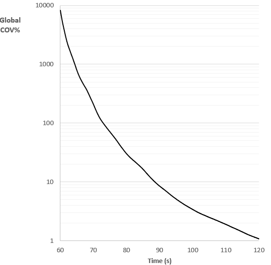
Time evolution of the global scalar field COV percent, as normalized by 0.000109 mol/L, the mean concentration in the vessel following the dye pulse.

In misclabel7, for the same system, we present the time-evolution of the local scalar field concentration, as extracted from the three virtual probes in the tank. This concentration data is recorded automatically by the solver in the probe.txt output files. As expected, the top probe immediately sees the first spike, which occurs about 5 seconds after the dye injection on the opposite side of the tank. The bottom probe is the last to detect any dye. With increasing time, the concentration at each probe location approaches the same value, which is equal to the mean dye concentration in the tank. Note that the top probe is the last probe to settle within 2% of the mean dye concentration. This convergence occurs after 105 seconds, corresponding to a 45 second blend time. 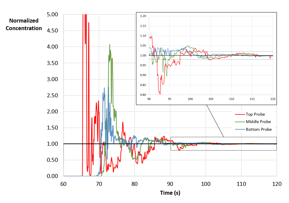This value is consistent with the blend time predicted from the time-evolution of the global COV presented above.

Time-evolution of the scalar concentration at each probe. Concentrations normalized by 0.000109 mol/L, the mean concentration in the vessel following the dye pulse. Inset presents the final 30 seconds of blending. Guide lines at +/- 2% are shown on the inset figure.

Since the global COV data is calculated over the entire flow volume, the prediction will necessarily include the last regions to blend. The global COV, in most cases, will therefore represent a more conservative blend time prediction between the two approaches. Missing from this global COV output, however, is precise insight into how the dye is actually distributed across the vessel over time. With probes, which have a known location, additional details related to the concentration distribution driving the reported global COV are immediately available.

In misclabel79, we compare the 95% blend time predicted blend time (extracted from the global COV) to the measured blend time across a range of fill heights and impeller speeds in the 500 L and 2000 L reactors. [1-2] The agreement is reasonable across all 18 reported operating conditions, in terms of both magnitude and trend. All simulations were executed on a desktop workstation with 2 Nvidia V100 GPUs. Each simulation took 2-5 wall hours to simulate between 1 and 5 minutes of agitation (which included the 1-2 minute initialization time).

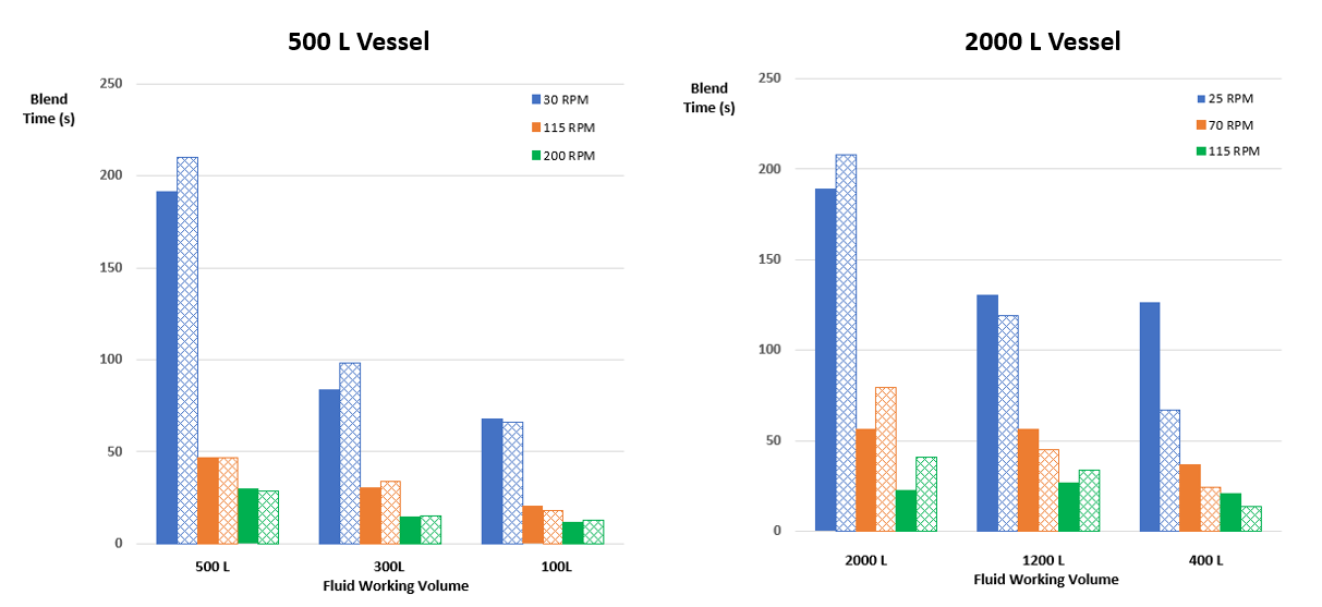
Measured blend time (solid bars) versus predicted blend times (patterned bars) across a range of operating conditions.

The largest difference between prediction and experiment occurred in the 2000 L vessel with a 400 L working volume operating with a 25 RPM impeller speed. We note that this system had the largest measurement uncertainty of any configuration, with experimentally blend time measurements ranging from 80 to 160 seconds. In this case, the average measured value was 126 seconds, while the solver predicted a blend time of 60 seconds. To understand this difference, we can compare these two values to predictions for literature correlations derived for similar systems. Following the work by Grenville [3], the blend time in a tall turbulent tank can be predicted from:

\[\theta_{95} = \frac{5.20 T^{1.5} H^{0.5}}{N D^2 Po^{1/3}},\]

where \(\theta_{95}\) is the 95% blend time, \(T\) is the tank diameter, \(H\) is the fluid height, \(N\) is the impeller speed, \(D\) is the impeller diameter, and \(Po^{1/3}\) is the impeller power number. The fluid height for this operating condition is 0.437 m, such that the blend time estimated from the correlation is 66 seconds. This estimate would corroborate the 60 second blend time predicted here.

Building the Multi Fluid Model

We now build a 10 L bioreactor system, as shown in misclabel8, which is agitated by a top-entry, off-centered low solidity hydrofoil impeller located near the tank bottom. Note that this system begins as two stratified fluids: the bottom 80% of the vessel volume is a protein surrogate, modeled as an aqueous solution of 11 wt % sodium chloride and 0.6 wt % sodium carboxymethylcellulose (CMC) solution. The density of the surrogate is taken to be 1080 kg/m³. Above this base surrogate, the top 20% of the vessel volume was filled with water, which has a density and viscosity of 1000 kg/m³ and 10^-6 m²/s. The water layer on the top of the vessel is modeled as a miscible fluid with a diffusion coefficient of 10^-9 m²/s. The impeller diameter is 0.086 m and spins at 338 RPM. The tank diameter and height are 0.21 m and 0.31 m, respectively, which corresponds to an aspect ratio of 1.5. A resolution of 300 is selected, which is expected to give a good prediction on impeller power number. We use the default Courant number of 0.1 with the default Van Leer flux limiter.

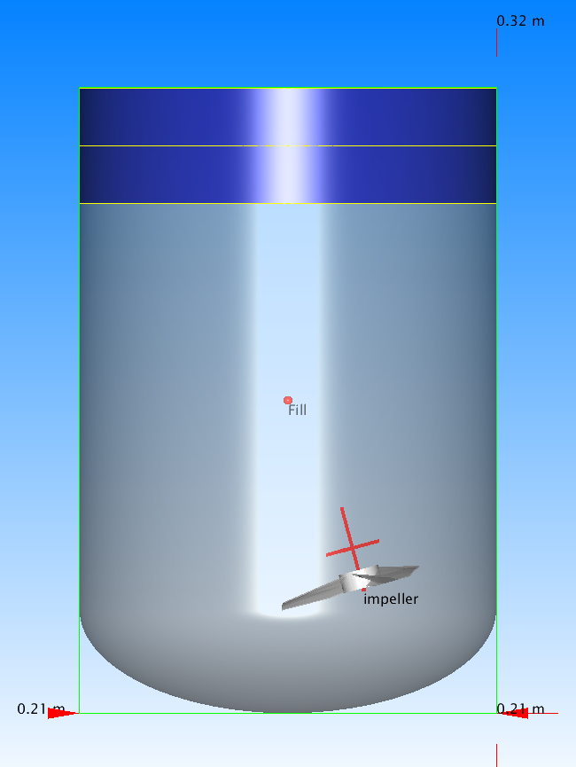
Set-up of the 10L bioreactor with two miscible fluids. The blue cylinder at the top of the vessel represents the initial water layer.

In misclabel9, which is adapted from the work of Benchabane and Bekkour [4], we present the variation in the protein surrogate viscosity as a function of strain and CMC concentration. At concentrations relevant here (<= 0.6%), the surrogate is shear-thinning and can be modeled as a Cross fluid. Superimposed on the experimental data is the rheology predicted for a 0.6% surrogate, which is developed using the parameters presented by the authors. Note that, over the range of shear rates relevant in this system, the surrogate viscosity is expected to increase from approximately 5.0x10^-5 m²/s near the impeller to approximately 1.0x10^-4 m²/s near the water interface. The experimental data also suggest that, to a first order, the viscosity of the surrogate is a linear function of CMC concentration in this low concentration limit. That is, across the relevant range of strain rates, the viscosity of the of the 0.4% CMC surrogate and 0.2% CMC surrogate are approximately 2/3 and 1/3 that of the 0.6% CMC surrogate.

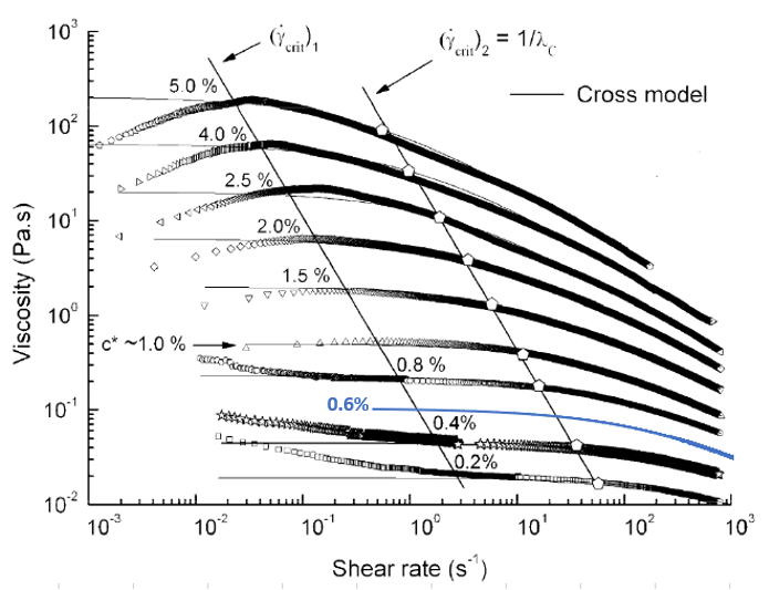
Protein surrogate viscosity as a function of strain rate and CMC concentration. Adapted from [4].

To properly capture these non-Newtonian and concentration-dependent effects, we use the custom fluid model shown in misclabel10. Note that this model is applied at every time-step to each voxel in the domain using the local fluid properties. In principle, since we are writing custom code, we can apply a more sophisticated mixing relationship to describe the effects of water concentration on local viscosity. In practice, however, this additional precision will be probably be small relative to the uncertainty in the actual fluid rheology and uncertainty measured blend time.

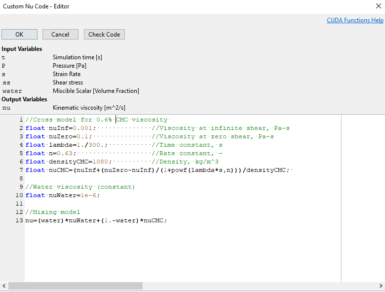
Custom rheology expression used to model combined effects of shear and concentration on viscosity

In misclabel12a, we show the effects of the custom fluid model in action early into a simulation. In the left pane, we show the water concentration which is still stratified. In the middle pane, we show the strain rate across the fluid. In the right pane, we show the local fluid viscosity. Near the impeller, where the CMC concentration is around 0.6% and the strain is around 300 1/s, the effective viscosity is around 5.0x10^-5 m²/s. Near the impeller, where the strain is on the order of 1 1/s, the viscosity is 2x higher. In the bulk of the water layer, which has not yet mixed, the viscosity is 1.0x10^-6 m²/s. Within the interface, where water is blending with the surrogate, intermediate viscosities are realized.

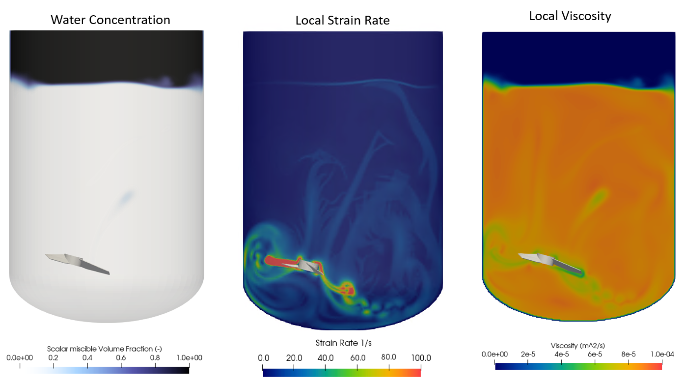
Custom rheology expression used to model combined effects of shear and concentration on viscosity

Note that the code automatically uses a volume fraction-averaged approach when computing the density within each fluid voxel:

\[\rho_{j}= \rho_w \gamma_j+\left(1-\gamma_j\right)\rho_p,\]

where \(\rho_j\) is the fluid density within voxel \(j\), \(\rho_w\) is the density of the pure water, \(\rho_p\) is the viscosity of the protein surrogate, and \(\gamma\) is the volume fraction of water within the voxel. This averaging occurs inside the solver using the user-defined fluid densities.

Analyzing the Miscible Fluid Blendtime

In the movie below, we show the time-evolution of the fluid velocity, viscosity, and water concentration. Despite the aliasing effects of the movie sampling frequency, the impeller is spinning at 338 RPM. [6] As required by the no-slip boundary condition, the fluid velocity next to the impeller is consistent with the impeller tip speed (1.52 m/s). Near the tank walls and interface, however, the velocity is much lower and ranges from 0.05 to 0.2 m/s. After 450 seconds of agitation, as a homogenized fluid, the viscosity varies from 4.0x10^-5 m²/s near the impeller to 7.0x10^-5 m²/s near the tank walls. These global variations are due to local variations in strain, and are consistent with the Cross model presented above.

Note that the blending process is similar to a one-dimensional melting process, wherein water at the interface is transported into the surrogate along the moving bottom boundary. Although very different from blending in turbulent systems, this linear blending behavior is consistent with recorded visual observations for this system. [6] The predicted power number for the impeller is 0.35, which is reasonable given the hydrofoil speed, configuration and rheology.

In misclabel12, we present the time-evolution of the water COV percent versus the number of impeller turns. This data calculated automatically and come directly from the miscible.txt output file. The 95% blend time is 468 s (2640 impeller turns), which is within 11% of the experimentally measured 95% blend time of 420 second (2370 impeller turns).

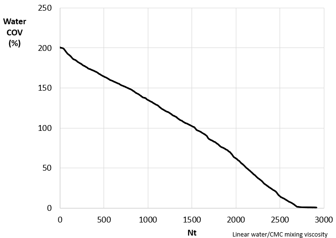
Evolution of water COV as function of impeller turns for the 338 RPM condition. The predicted 95% blend time is 2640 impeller turns (468 seconds). The measured 95% blend time is 2370 impeller turns (420 seconds).

To test the robustness of the model, we re-ran this system at impeller speeds of 290 RPM, and 494 RPM. The predicted blend-times, along with the experimentally measured values are presented in misclabel13. Note that, for each system, the time-evolution of the water COV had a linear decay similar to that shown in Figure 3. The order-of-magnitude differences in blend time associated with 0.5x to 1.5x changes in impeller speed are stark, even for a non-Newtonian fluid. The effects of density-driven stratifications are clearly informing process outcomes. It is encouraging, however, to see the model correctly capture this experimental observation. The agreement gives confidence to the accuracy of the integration schemes, control over numerical diffusion, and the robustness of the rheology model.

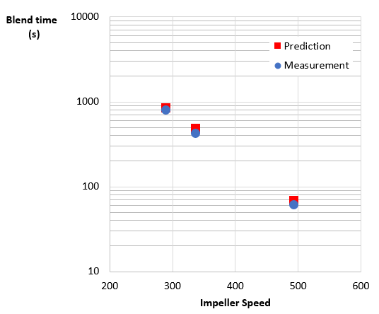
Predicted versus measured blend time for 290, 338, and 494 RPM operating speeds. Adapted from Ref. [6].

References

[1] GE Healthcare Engineering characterization of the single‑use Xcellerex XDR‑500 stirred‑tank bioreactor system. Application note KA4969250918AN

[2] GE Healthcare. Engineering characterization of the single-use Xcellerex XDR-2000 stirred-tank bioreactor system. Application note 29243481AA

[3] Grenville, R. K. and Nienow, A. W., 2003, Blending of Miscible Liquids. Handbook of Industrial Mixing.

[4] Benchabane, A. and Bekkour, K, 2008, Rheological properties of carboxymethyl cellulose (CMC) solutions. Colloid and Polymer Science volume 286, 1173 .

[5] For this three-bladed hydrofoil, the blade pass frequency is three times the impeller speed: 3 blades x 338 rotations/minute=1014 blade passes/minute. The image output frequency was 10 seconds, which coincidentally corresponds to exactly 1014 x 10/60 = 169 blade passes between snapshots in this configuration. The integer number of blade passes between snapshots means the moving impeller will appear at the same location in each frame.

[6] Zhao, Y., Finch, B. A., Hale, D. A., 2018, Mixing of Stratified Miscible Liquids in an Unbaffled Tank with Application in High Concentration Protein Drug Product Manufacturing, Ind. Eng. Chem. Res. 57, 3397-3409