Flow in the Trailing Vortex of an Impeller

Although M-Star CFD is an inherently transient solver, it’s straightforward to predict the time-average flow field and compare it to measured particle image velocimetry (PIV) data and laser doppler anemometry data. In Fig. 1 below, we compare the instantaneous flow field to the time-average flow field after 18.65 seconds agitation for a 10-cm Rushton impeller spinning at 200 RPM in water. Time-averaging was initiated after 5 seconds of agitation, allowing the system to reach quasi-steady state before data collection. By this point, from a data validation perspective, the time-average flow field is sufficiently converged.

A movie showing the time-evolution of this data is available

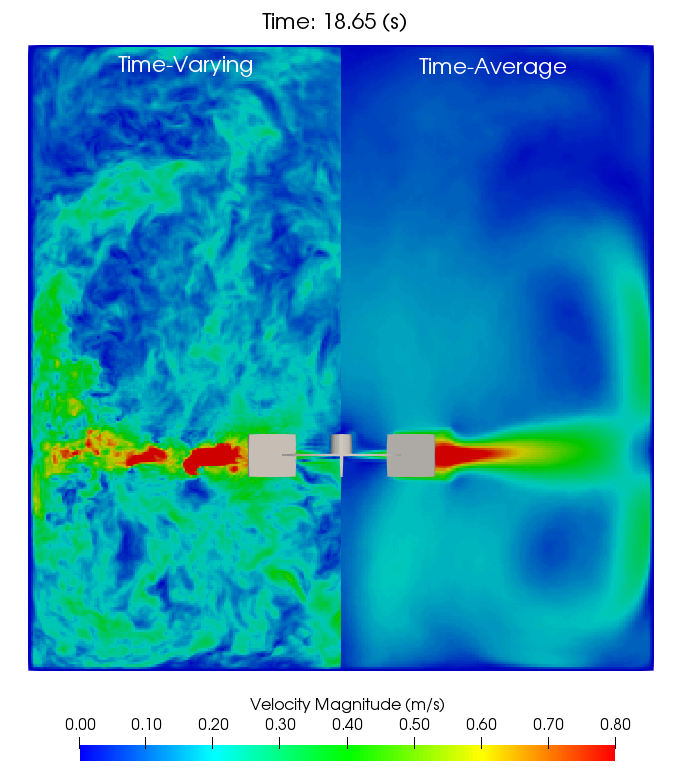
(left) Time-varying velocity field. (right) Time-average velocity field

The open literature contains an abundance of PIV and LDA data for systems like this, describing the variation in the mean x, y, and z-velocities at various position across the tank. Here we will use the LDA data reported by Wu and Patterson, which was obtained from the same system modeled in the figure above.:raw-latex:cite{Wu} A summary of the experimental data is presented in wudata. Each subfigure represents a family of curves, describing the variation in fluid velocity with radial location at a set axial position relative to the impeller disc. The mean velocity in the radial, tangential, and axial directions, normalized by the impeller tip speed, are reported at each point. Note that, while the radial position is reported in centimeters, the axial position above and below the impeller are normalized by the width of the impeller blade.

Summary of mean-flow LDA data from Wu and Patterson [Wu]

In axialflow, we compare the mean axial flow velocity measured from LDA (points) to continuous profiles predicted from M-Star (lines). The purple and black lines correspond to two axial traces at the same radial location, but on opposite sides of the impeller. In each subplot, the +x direction corresponds to axial distance away from the bottom of the tank. The axial trace closest to the impeller is positioned 5 cm away from the tank center. The axial trace furthest from the impeller (and closest to the tank wall) is positioned 10.5 cm away from the tank center. Across all available data points, the agreement between simulation and experiment is comparable to the variance across the tank cross-section and the measurement uncertainty.

Mean axial flow along an axial trace at multiple radial locations. Predictions (points) obtained from LDA [Wu]. Simulation (lines) obtained from M-Star CFD

In radialFlow, we compare the mean radial flow velocity measured from LDA (points) to continuous profiles predicted from M-Star (lines). Again, the purple and black lines correspond to two axial traces at the same radial location, but on opposite sides of the impeller. Across all available data points, the agreement between simulation and experiment is comparable to the variance across the tank cross-section, measurement uncertainty, and the readability of the charts.

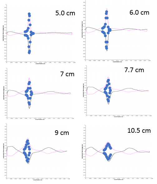
Predictions (points) obtained from LDA [Wu] Simulation (lines) obtained from M-Star CFD

Mean radial flow along an axial trace at multiple radial locations. Predictions (points) obtained from LDA [Wu] . Simulation (lines) obtained from M-Star CFD

We conclude in tanFlow by comparing the measured mean tangential flow velocity to profiles predicted from M-Star. Again, the agreement is very good.

Mean tangential flow along an axial trace at multiple radial locations. Predictions (points) obtained from LDA [Wu]. Simulation (lines) obtained from M-Star CFD

[Wu] (1,2,3,4,5)

Wu, H., and G. K. Patterson. “Laser-Doppler measurements of turbulent-flow parameters in a stirred mixer.” Chemical engineering science 44.10 (1989): 2207-2221.