 Add Geometry
Introduction
In M-Star CFD, the parent-child relationship is a foundational concept used to structure simulations.
Parents define the how and what of a simulation. These properties include what properties are associated with any static boundary conditions, how moving objects are expected to move through a system, what types of particle sets will be included in the simulation, and what types of species will be considered.
Children define the extent and shape of the parents. These properties include the extent of the static boundary geometry, the shape of the moving impeller, the location a particle set will be injected into the system, and the location where a species will be introduced into the system. Sometimes the children represent physical geometry, as in static and moving bodies, in other cases the children are simply regions of space where these properties will be applied.
Although not all parents need children geometry, all children geometry must have a parent.
Access
Children geometry are most commonly added to parents via the Add Geometry window. A parent must be created before a child geometry can be added to it. There are two ways to access the window:
The Add Geometry window will open automatically when you define a new parent with the Create menu. The child geometry is most often attached to a parent when the parent is first created.
Launch the window manually by clicking on Add Geometry in the Context-Specific Toolbar. The toolbar will appear when you select the previously-created parent component you wish to define, and here you will find the Add Geometry command.
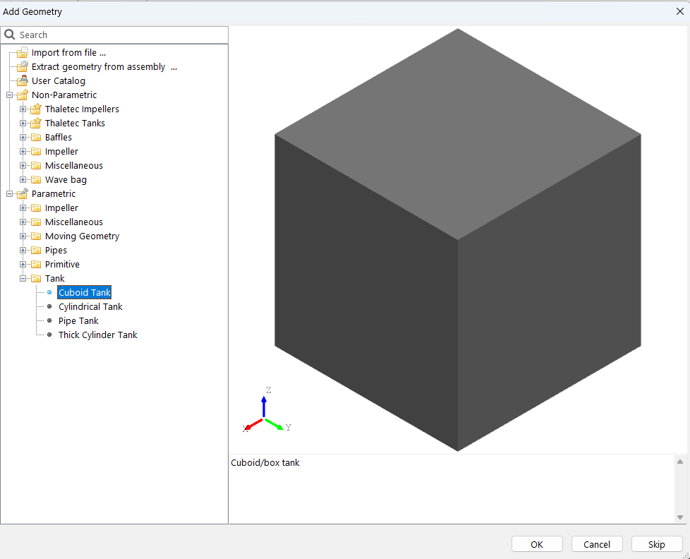
Add Geometry Window
The Add Geometry window is where you select your child geometry.
 Import from file
Import a CAD part file from an external CAD program on a part-by-part basis.
M-Star supports the following geometry formats for import:
*.stl: STL Mesh files; uses triangles to describe the surface geometry of a three-dimensional object.*.obj: OBJ Mesh files; an open 3D graphics format that represents geometry as a list of vertices.*.iges, *.igs: IGES Boundary representation files; a vendor-neutral file format used in CAD systems.*.step, *.stp: STEP Boundary representation files; an ISO standard exchange format used for 3D modeling.*.x_t, *.x_b: Parasolid CAD files
Tip
Use the Import CAD Assembly Workflow function to import files composed of multiple parts (or sub objects), such as tanks and impellers.
Be aware of object location in space. Sometimes imported geometry may have an unexpected origin. In general it is suggested to keep the object close to world 0,0,0 when importing the geometry.
Be aware of the scale of the imported geometry. STL mesh files do not contain any data about units, so you will be prompted at import time to specify what the units are.
Explode: Explode an imported geometry after it is imported into multiple sub-objects.
 Extract Geometry from Assembly
Extract individual parts from an existing CAD assembly file. A CAD assembly file is a file that contains multiple CAD parts. This workflow is useful if you have already integrated your CAD geometry—such as your static and moving bodies—in a single CAD assembly file.
This option launches the Assembly Explorer form which allows you to select and extract individual child geometry from the CAD file. Select the geometry you want to extract from the assembly and click OK.
M-Star supports the following file formats:
*.iges, *.igs: IGES Boundary representation files; a vendor-neutral file format used in CAD systems.*.step, *.stp: STEP Boundary representation files; an ISO standard exchange format used for 3D modeling.*.x_t, *.x_b: Parasolid CAD file
Import Deforming Meshes
The option will only appear when there is a Moving Body in the Model Tree. The Import Deforming Meshes command is used to load a set of externally generated mesh files that define a deforming moving body. It provides maximum flexibility for modeling complex motion but requires careful preparation of the input data.
The option allows you to load a series of STL files, each representing the deforming geometry at a specific time point. The solver interpolates the mesh between these time points to produce smooth, continuous motion. Each STL file must correspond to a single time point in the simulation, and the file name must include the associated time stamp (for example, Deforming_Mesh_3.15.stl represents the geometry at t = 3.15 s). The number of vertices, edges, and faces must remain identical across all STL files to ensure correct interpolation, and the solver relies on the time values provided by the user to guide interpolation between files. A sample set of mesh files is provided in the link below—these files are distributed as a zipped archive and must be unzipped before loading.
Download Sample File: Deforming Mesh STL
Download Sample File: Mesh Files
Note
Only one deforming mesh may be added to a moving body.
 Parametric Catalog
In the Parametric Catalog you find the options for child geometry in which you can fully customize the shape and topology of the geometry. All the parameters used to define the geometry can be edited by the user. These parameters include vessel shapes, head types, impeller blade and angles, and pipe diameters and bends.
For a complete list of the parametric geometry, see the Parametric Catalog.
 Non-Parametric Catalog
In the Non-Parametric Catalog you will find non-parametric options for child geometry. Non-parametric geometry parameters are not editable, they can only be scaled uniformly. These include geometries typical of vendor systems.
For a complete list of the non-parametric geometry, see the Non-Parametric Catalog.
 Add Fill Point
M-Star CFD uses a 3D flood fill algorithm to generate region tags over the lattice at runtime. Each fill point defines the origin of a volumetric expansion that marks all reachable voxels until blocked by static geometry or the simulation bounding box. The resulting tagged regions are central to several workflows, including defining the active region stored in memory, initializing disconnected regions with different fluids, scoping global variable reductions, and defining particle or scalar injection locations.
After defining static and moving bodies (whether single part or multiple components), fill points are placed to seed the flood fills. These points should be in the bulk fluid away from any static or moving body geometry. At time zero, the solver expands from each fill point until reaching static boundaries or the bounding box, tagging connected regions and distinguishing them from disconnected ones. This approach automatically decomposes the system geometry into distinct regions, without manual preprocessing. Conceptually, the 3D flood fill behaves like an expanding balloon: it grows outward from the fill point, conforming to the geometry and stopping at boundaries. Because this decomposition happens algorithmically at runtime, there is no need to import separate geometries, construct region masks, or duplicate models. The flood fill always produces the same output—a tagged set of lattice voxels—but the meaning of those tags depends on where the fill point is defined.
Fill Points on Free Surface and Two-Fluid Configuration
In a two-fluid (VOF) model, fill points initialize disconnected regions with different fluids, assigning one phase to each region at the start of the simulation. When a fill point is added under a Free Surface or Immiscible Two Fluid configuration, the resulting tagged region defines the initial fluid assignment at the start of the simulation. The 3D flood fill is performed once at time zero.
Each tagged region can be associated with a specific fluid type, enabling disconnected regions to begin with different initial phases. For example, if two compartments are separated by walls, one region can be initialized with Fluid 1 while another is initialized with Fluid 2. This provides precise control over the initial conditions in multiphase systems, ensuring that each region starts with the correct fluid configuration before the solver advances in time.
Fill Points for Particles and Scalars
When a fill point is used under scalar field or particle parent, the resulting tagged region behaves like an algorithmically defined child geometry, created once at time zero. The tagged region defines where additions occur, ensuring that particles or scalars are introduced only within the intended subregion. Because the tagged regions are generated directly by the 3D flood fill, they adapt automatically to the as-built geometry, removing the need to manually construct additional geometry or region masks.
Fill Points for Global Variables
When a fill point is used under global variables, the resulting tagged region behaves like an algorithmically defined child geometry, created once at time zero. The tagged region the flood fill restricts reductions (e.g., integrals or averages) to the tagged region only. That is, the tagged region specifies where reductions are applied, limiting integrals, averages, or totals to that volume. Because the tagged regions are generated directly by the 3D flood fill, they adapt automatically to the as-built geometry, removing the need to manually construct additional geometry or region masks.
Fill Points for Porous Media and UDF Regions
When a fill point is used under porous media and UDF Regions, the resulting tagged region behaves like an algorithmically defined child geometry, created once at time zero. For Porous Media, the tagged region specifies the volume occupied by the porous media. For UDF Regions, the tagged region specifies the interior of the geometry. Because the tagged regions are generated directly by the 3D flood fill, they adapt automatically to the as-built geometry, removing the need to manually construct additional geometry or region masks.
Location
The Add Geometry form is found on the following context-specific toolbars:


