Optimize Blend Time
See the associated training video – Optimization Example
This example demonstrates how you can interface the scipy.optimize library with M-Star. This example uses the global optimization routines available in scipy to optimize the Y location of a Rushton impeller in a baffle cylindrical tank. This is a global optimization since the search area is relatively large. The impeller location is set allowed to be in the range [0, 0.5] meters. This allows the impeller to placed anywhere along the entire height of the tank. No other variables are allowed to change.
In the script we invoke 2 different optimizers to demonstrate the varying behavior of these algorithms. The first is the minimize_scalar and second method is the shgo method. You can change the method by comment/uncommenting the appropriate code blocks in the script.
Create a new directory and download the following items.
Download the script here –
mstaroptimize.pyDownload the base document here –
simpleOptimize.msb
How it works
The scipy optimizers are generally called in this way –
res = minimize_scalar(runCase, bounds=(0, 0.5), method='bounded', options={'maxiter':100})
Here the runCase method is defined as a function that takes in a single parameter (Y location of impeller) and outputs a single value (acheived blend time). To do this, the method does the following:
first loads in a base MSB file (simpleOptimize.msb)
changes the Y location of the impeller
exports the files to a numbered case directory
run-N, saves the msbruns the solver
processes a Stats file to determine the resulting blendtime
This particular msb file was set up to inject the scalar after 10s of spin up time. The simulation then stops when the case is sufficiently blended. This is done using the Stop Condition input on the Simulation Parameters. This helps save evaluation time.
The minimize_scalar optimizer function will then call this runCase function, varying the input value for the Y location and keeping track of the results. The result of the optimize method generally has all the function evaluation inputs/results, as well as other algorithm specific values.
To run the script –
python mstaroptimize.py
The below plots show the behavior of these optimize algorithms. Y impeller location is on the independent axis. Blend time is on the dependent axis.
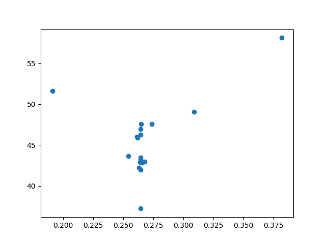
Fig. 62 minimize_scalar method. It looks like it did not sample the full space much before deciding to attack a local minima.
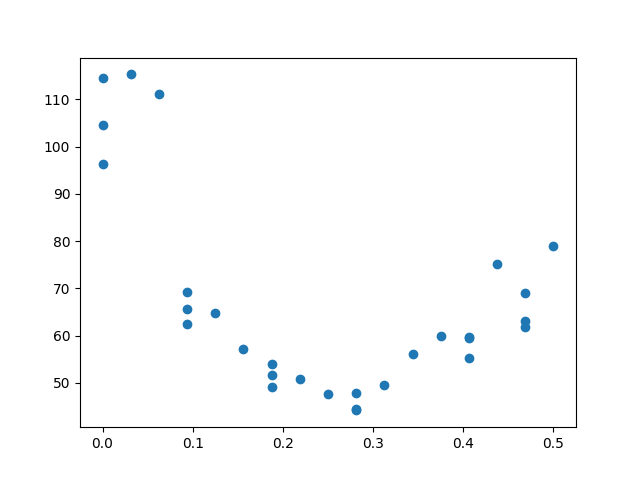
Fig. 63 shgo method. This method sampled the global space more, but did not attack local minima as much as the previous method.