Scalar Field¶

Introduction¶

Scalar fields are continuous field variables that evolve according to the advection-diffusion-reaction equation. Within this framework, the time-evolution of the local scalar field concentration is governed by the host fluid’s motion through advection, the local concentration differences causing diffusion, and the processes occurring locally as reactions. Scalar fields are typically used to model species mixing and transport processes, like blending and dispersion; but this feature is also useful when modeling interfacial mass transfer processes, such as dissolution, dissolved gas transfer, and solids drying applications.

Download Sample File: Scalar Field

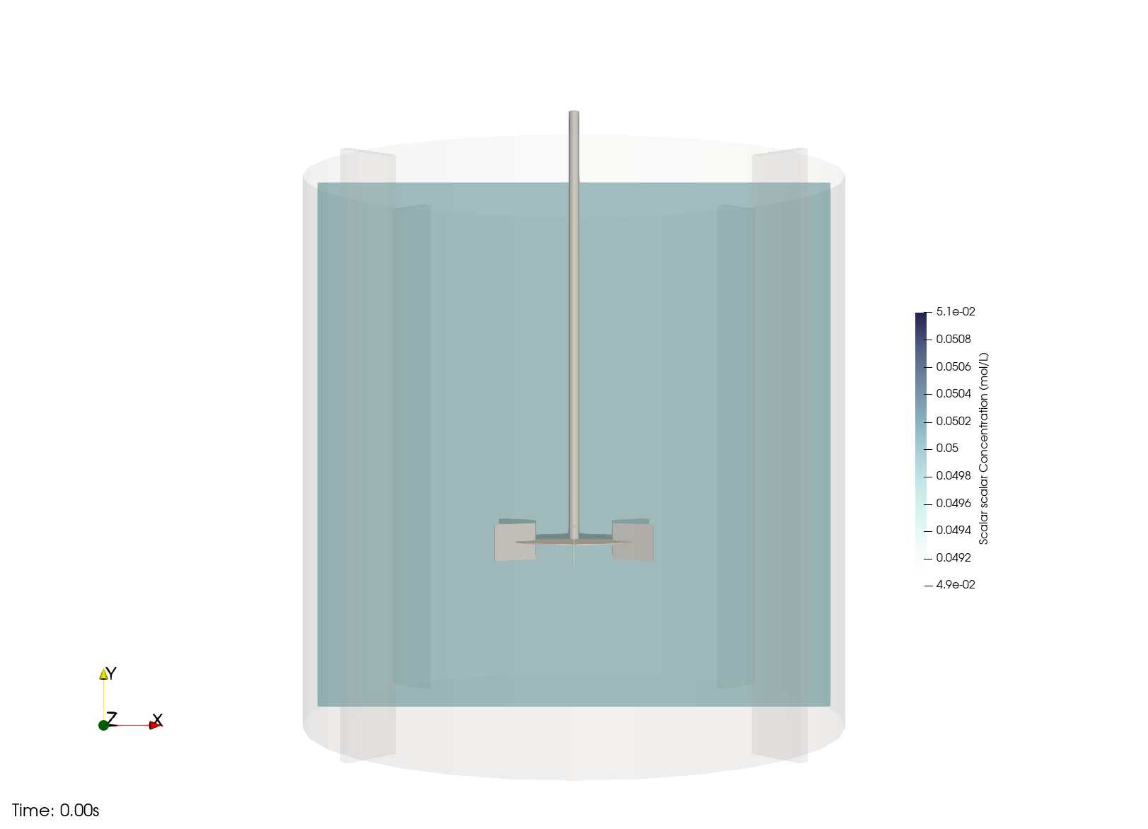
In the above Scalar Field model, the figure on the left shows a time-evolving velocity field in a 2000 L bioreactor. The figure on the right shows the time evolution of glucose concentration following a bolus addition at the top of the vessel. The fluid transport and scalar transport processes are solved in tandem. The glucose is homogenized over time due to the ongoing effects of advection and diffusion.

Scalar fields represent a continuous scalar value, or species concentration, defined at all points across the fluid domain. This means that all lattice voxels possess a local scalar field concentration (including zero concentration). Each scalar field represents a single species, such that the local value/magnitude of the scalar field characterizes the local concentration of the species represented. The magnitude of the species can be can be mensurated in moles, volume, or mass.

Scalar fields can be coupled to the fluid to inform the local fluid density and viscosity. They can also occupy the particles; they can be coupled to bubbles or particles to describe mass transfer processes and reaction/dissolution processes. As such, species contained within the fluid can interact with species in the particles via particle-scalar coupling. Multiple scalar fields can participate in reactions, with local reaction rates informed by the local fluid properties and species concentrations.

Scalar fields are defined using the parent-child relationship. The parent defines the overall properties of the scalar field, such as scalar field representation, species diffusion coefficient, advection scheme, scalar field density, etc. The parent also defines how species are added to the system along the boundary condition surface and/or within any child geometry. Children geometry define the shape, geometry, and extent of any localized species addition/removal during the simulation. Children geometries can be added to scalar family sets via the Add Geometry form on the context-specific toolbar.

Download Sample File: Scalar Recirculation

In the above Scalar Recirculation model, the figure on the left shows a time-evolving scalar field in a recirculating vessel. The recirculation intake is positioned on the bottom left of the vessel, while the return is positioned on the top right. The figure on the right shows the time evolution of scalar concentration realized at the recirculation intake. The fluid transport and scalar transport processes are solved in tandem.

The time evolution of each scalar field within each voxel is defined by the advection-diffusion equation reaction:

\[\frac{d c_{i j}}{d t}=D_i\left(\nabla^2 c_{i j}\right)-\nabla \cdot\left(\vec{V}_j c_{i j}\right)+\dot{n}_{i j}+\dot{r}_{i j}\]

where \(c_{i j}\) is the concentration of species \(i\) within fluid voxel \(j\), \(D_i\) is the species diffusion coefficient, \(\vec{V}_j\) is the fluid velocity, \(\dot{n}_{i j}\) is the local gas-liquid mass transfer rate, and \(\dot{r}_{i j}\) is the local aqueous reaction rate. The advection-diffusion equation is advanced in tandem with the fluid flow model, using the same fluid lattice and simulation time step. As such, the velocity \(\vec{V}_j\) evoked in the equation is the local and instantaneous fluid velocity, while the species concentration \(c_{i j}\) computed from the equation can be used as input to the flow model. In this manner, changes to the local fluid density or rheology due to changes in the local species concentration can be modeled explicitly via a custom fluid viscosity UDF.

In principle, the code can support an arbitrary number of scalar fields and associated species concentrations. In practice, however, each field introduces a 10–20% reduction in runtime, relative to a system with no scalar fields. Although these effects can be minimized by selecting a larger update frequency, effort should be made to minimize the number of scalar fields included in the model.

Specifying Species Concentrations¶

Species can be added to a scalar field using (i) a children geometry, (ii) an inlet boundary condition, (iii) a background injection, (iv) reaction kinetics, or (v) interfacial mass transfer.

A child geometry injection represents the addition of species onto the scalar field within a sub-volume of the fluid domain. Fluid flow sweeps this added species from the initial injection region within the child geometry to other regions in the system.

An inlet boundary condition represents the concentration of species along the boundary condition surface. Flow through the boundary condition advects species from the initial injection region along the boundary condition surface to other regions in the lattice.

A background injection produces a uniform distribution of species across the full fluid field. This addition, which is applied at the start of a process, represents a system with an initially well-mixed concentration.

Reaction kinetics can be used to produce (or consume) species across the scalar field. Reactions are modeled on a voxel-by-voxel basis. The ongoing effects of advection and diffusion move species produced in one voxel to other regions of the lattice.

Interfacial mass transfer is used to model mass transfer across a solid/liquid, liquid/liquid, or gas/liquid interface. For two-fluid Eularian-Eularian immiscible fluids, this transfer is handled via the scalar transfer functionality. For a system with Lagrangian particles, this is handled via particle scalar coupling.

When using a child geometry injection, users have three options for adding geometry to the particle parent: (i) via the Add Geometry form, which opens automatically when a new particle parent is created; (ii) by importing geometry through the Assembly Explorer; or (iii) by importing geometry from a spreadsheet. See the Geometry page for more details.

For an already-existing parent component, you can add children via the Add Geometry command found on the Context Specific Toolbar. Children geometry can also be extracted from an assembly file.

Property Grid¶

`General`¶

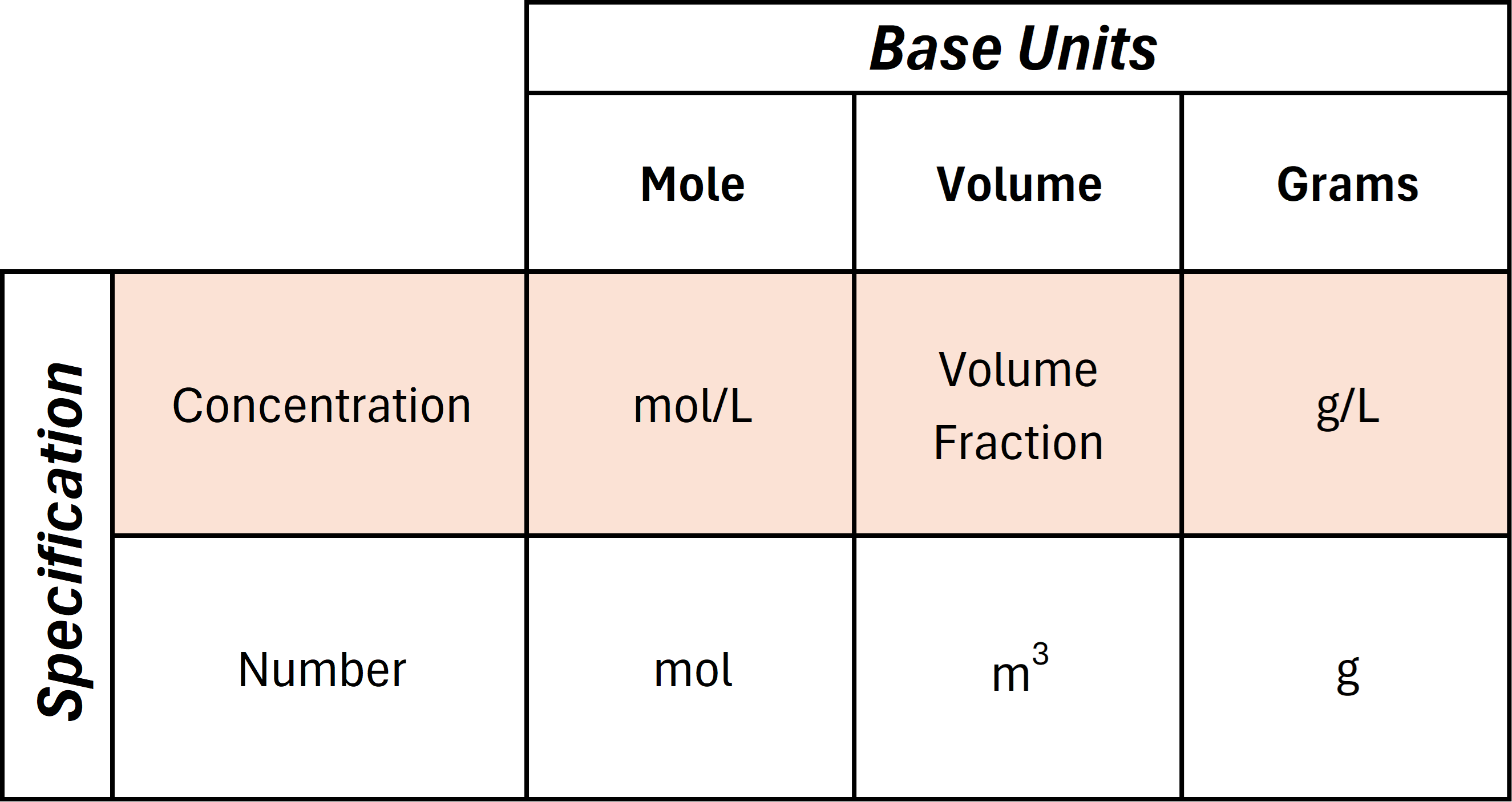
Base Units

This parameter defines the base unit used to characterize the local species concentration. The base unit of the species can be specified in terms of moles, volume, or mass.

Moles

Defines the local species concentration in terms of moles. Within this framework, species concentrations will be defined in terms of mols/liter and any species addition or removal rates will be defined in terms of mols/second. This unit representation is commonly used when modeling reacting systems.

Volume

Defines the local species concentration in terms of volume (\(m^3\)). Within this framework, species concentrations will be defined in terms of volume fraction relative to the fluid. Any species addition or removal rates will be defined in terms \(m^3\)/second. This unit representation is commonly used with passive mixing and systems with density-driven stratifications. The volume representation is incompressible, meaning the maximum volume fraction realized in each voxel will not exceed one. This limit on occupancy applies to systems with multiple scalar fields, as the sum of all volume fractions in a given voxel will not exceed one.

Fluid Density Option

This option allows the user to specify a unique density associated with the scalar field. Within each voxel, the effective local density \(\rho_e\) is then calculated from the corresponding local scalar field volume fraction \(\alpha_s\) via:

\[\rho_e = \rho_f (1 - \alpha_s) + \rho_s (1 - \alpha_s)\]

where \(\rho_f\) is the density of the base fluid. This functionality is useful when modeling two-fluid miscible systems with differing densities. This workflow is illustrated in the Multi Fluid Model.

Density: The density of the fluid represented by the scalar field. Larger density differences between the two fluids can lead to stratification and long blend times. See reference publication.

Mass

Defines the local species concentration in terms of mass. Within this framework, species concentrations will be defined in terms of mass/liter and any species addition or removal rates will be defined in terms of mass/second. This unit representation is commonly used when modeling dissolving systems.

Diffusion Coefficient Type

There are two options for defining the species diffusion coefficient: Constant and UDF.

Constant

The diffusion coefficient is a constant value that is uniform through the simulation domain.

Diffusion Coefficient: m ² /s | Diffusion coefficient of the scalar through the base fluid. Typical liquid-liquid diffusion coefficients range from \(10^{-9}\) to \(10^{-8}\) \(m^2/s\), depending on temperature and composition. Typical gas-gas diffusion coefficient ranges from \(10^{-6}\) to \(10^{-5}\), again depending on temperature and composition.

UDF

The diffusion coefficient is a user-defined function that can be time-varying and non-uniform.

Diffusion Coefficient UDF

m ² /s | This UDF defines the local species diffusion coefficient. One output must be defined within the UDF: a floating-point variable named D. This output variable defines the local species diffusion coefficient within the fluid. This is a voxel-based local UDF, calculated on a voxel-by-voxel basis using the local fluid properties.

Download Sample File: Diffusion Coefficient

Note

Scalar fields can be susceptible to numerical diffusion. Numerical diffusion occurs when the simulated fluid presents a higher diffusivity than the physical fluid. The effects of numerical diffusion can be minimized by reducing the simulation resolution, applying a flux limiter, or increasing the scalar field update interval. When running scalar fields in a simulation, resolution tests should be performed to ensure that the effects of numerical diffusion are negligibly small. This point is discussed in Application of flux limiters to passive scalar advection for the lattice Boltzmann method

If Immiscible Two Fluid is selected, the following setting will launch:

Phase Containment

This setting specifies which fluid hosts the scalar field. Unless Interfacial Scalar Transfer is active, the scalar field will remain contained within the selected fluid phase throughout any advection and diffusion processes. Users can select either Fluid 1 or Fluid 2 as the host fluid for the scalar field.

Off: No phase containment.
Fluid 1: If selected, this fluid hosts the scalar field.
Fluid 2: If selected, this fluid hosts the scalar field.

`Initial Background Value`¶

This parameter defines the initial concentration of the species across the scalar field. The addition is applied at the start of a simulation and represents an initially well-mixed distribution.

Specification: This parameter defines the units of measure applied to the background concentration. The specification can be either (i) a concentration or (ii) a number. The base unit defines which unit to apply to the specification. The relationship between the specification, base unit, and corresponding background concentration unit is summarized in the following table:

Initial Background Value UDF

base units | This UDF defines the initial species background concentration. These values will be assigned uniformly to all fluid voxels. This is a System UDF.

../../../_images/Sample-File-Initial-Background-Concentration.png

Download Sample File: Initial Background Value

If a Free Surface is present, the following section will launch:

`Free Surface Boundary Condition`¶

Flux Option

This setting defines the scalar flux boundary condition at the free surface. By default, the free surface acts as a zero-flux boundary condition, implying that species does not cross the interface. Alternatively, a non-zero-flux value can be specified, implying that scalar is transported across the interface. This interfacial transport rate is modeled on a voxel-by-voxel basis and can be a function of the local fluid properties, the local species concentration, and any global variables or parameters.

No Flux

No flux across the free surface interface.

Automatic

Convective flux across the free surface interface is modeled using a semi-empirical convective mass transfer coefficient:

\[\dot{q}'' = k_l(S_s C_g - C_l)\]

where \(\dot{q}''\) is the scalar flux, \(k_l\) is the local convective mass transfer coefficient, \(S_s\) is the solubility of the gas in the (empty) headspace, \(C_g\) is the concentration of species in the (empty) headspace, and \(C_l\) is the local concentration of the species in the fluid. The units on the flux and concentration are set by the base units. The local convective mass transfer is calculated from the local Sherwood number, \(Sh\), via:

\[Sh \equiv \frac{kl \Delta x}{D} = CR e^{1/2} Sc^{1/3}\]

where \(\Delta x\) is the lattice spacing, \(D\) is the scalar diffusion coefficient, \(C\) is a semi-empirical cofactor, \(Re\) is the local Reynolds number, and \(Sc\) is the local Schmidt number. The local Reynolds number is calculated from:

\[Re = \frac{V \Delta x}{\nu}\]

where \(V\) is the local fluid velocity and \(\nu\) is the local kinematic viscosity. The diffusion coefficient \(D\) and kinematic viscosity \(\nu\) are set to user-defined values. Likewise, the local fluid velocity \(V\) and local species concentration \(C_l\) are calculated at runtime. The corresponding semi-empirical co-factor \(C\), dimensionless solubility \(S_s\), and (empty) headspace concentration \(C_g\) are user-defined.

Cofactor: dimensionless | Semi-empirical co-factor linking local Sherwood number to local Reynolds number and Schmid number. This parameter is typically between 0.1–1. See additional resources.
Dimensionless Solubility: dimensionless | Dimensionless solubility of the species in the empty headspace.
Head Space Concentration: mol/L | Concentration of the species in the empty headspace. The headspace concentration is assumed to be constant and well-mixed.

UDF

Transport across the interface is modeled via a user-defined function.

Interface Flux UDF

mol/(m ² \(\cdot\) s) | This UDF defines the species flux rate along the free surface interface. One output must be defined within the UDF: a floating-point variable named flux. This output variable defines the local interfacial species transport rate. Positive values imply flux entering the fluid. Negative values imply flux leaving the fluid. This is a voxel-based local UDF, calculated on a voxel-by-voxel basis using the local fluid properties. The flux specified in this UDF will only be applied along cells interacting with the free surface interface.

Download Sample File: Injection

If a child geometry is present, the following section will launch:

`Child Geometry Injection`¶

This parameter defines how species concentrations are modified inside the child geometry attached to the scalar field parent. Options are available to specify a set species concentration or a set species addition/removal rate. These values can be defined to occur either (i) across the interior volume of the child geometry or (ii) along the surface of the child geometry.

Specification

This parameter defines the units of measure applied to the species concentration. The specification can be either a concentration (per unit volume), a number, or a rate. The base unit defines which unit to apply to the specification. The relationship between the specification, base unit, and corresponding species concentration unit is summarized in the following table:

Per Unit Volume: Species addition is defined on a per-volume basis (concentration). The injection specification may be mol/L, volume fraction, or g/K, depending on the base units. This option is useful when modeling two miscible fluids with a set initial configuration.
Number: Species addition is defined on a number basis. The injection specification may be mol, m ³, or g, depending on the base units. This option is useful when modeling pulse additions of species to the system.
Rate: Species addition is defined on a rate basis. The injection specification may be mol/s, m ³ /s, or g/s, depending on the base units. This option is useful when modeling feed additions of species to the system.
UDF: Species addition is defined on a per-volume basis (concentration) per a user-defined expression.

Injection Location

This parameter defines where the species addition/removal will occur with reference to the child geometry.

Inject In Volume: The scalar boundary condition is imposed on all points contained inside the geometry.
Inject At Surface: The scalar boundary condition is imposed on the surface of the child geometry.

Child Geometry Value UDF

base units | This UDF defines how the species concentration will be added (or removed) from the system along the child geometry. The behavior of the system is informed by the injection specification. The UDF output units are determined by scalar field background specification. This can be either a System UDF or a Local UDF, depending on the Child Geometry Injection Specification.

Download Sample File: Child Geometry UDF

If the Child Geometry Injection Specification is set to Per Unit Volume (concentration) or Number, the values defined in the UDF will overwrite any existing scalar field values within (or along) the child geometry. When applied at the start of the simulation, it can establish a non-uniform initial species distribution. When applied later, it can simulate a bolus-type species addition. This configuration uses a System UDF.

If the Child Geometry Injection Specification is set to Rate, the UDF-defined rate will be superimposed onto any existing scalar field values within (or along) the child geometry. The UDF specifies the rate at which the local species concentration changes over time. This setup models processes like pouring, where an ongoing addition supplements the local species concentration. This configuration also uses a System UDF.

If the Child Geometry Injection Specification is set to UDF, the values defined in the UDF will overwrite any existing scalar field values within (or along) the child geometry. The UDF defines the local and instantaneous concentration across the child geometry over time. One output must be specified: a floating-point variable named {scalar}, where {scalar} is the dynamic name of the scalar field. This configuration uses a local UDF, calculated on a voxel-by-voxel basis within the child geometry using local fluid properties.

Injection Time Span

This setting defines the duration of the child geometry addition.

Entire Simulation

Maintains the Child Geometry UDF over the entire simulation. The UDF will be evaluated at each simulation time step.

Impulse

Applies the Child Geometry UDF at a single time step. The UDF will be evaluated once at this set impulse time.

Injection Impulse Time: Injection Impulse Time.

Time Window

Applies the Child Geometry UDF over a user-defined time window. The UDF will be evaluated over the duration of this time window.

Injection Window Start: Injection Window Start.
Injection Window Stop: Injection Window Stop.

Delayed Start

Following an initial delay, maintains the Child Geometry UDF over the entire simulation. The UDF will be evaluated at each simulation time step later than the time specified here.

Injection Window Start: Injection Window Start.

UDF

Offers a user-defined start and stop time.

Injection Start Time UDF: s | This UDF defines the time at which to begin the addition process within the child geometry. This is a System UDF.
Injection Stop Time UDF: s | This UDF defines the time at which to stop the addition process within the child geometry. This is a System UDF.

Download Sample File: Injection Start & Stop Time

If a moving child geometry is present, the following section will launch:

`Moving Injection Condition`¶

Moving Child Geometry Value UDF

Download Sample File: Moving Child Geometry UDF

If a static inlet or outlet is present, the following section will launch:

`Static Inlet Outlet Boundary Conditions`¶

{Inlet/Outlet} Boundary Condition Type

This parameter defines which scalar field values or fluxes will be applied at each static inlet/outlet. Inlet and outlet boundary conditions are defined along two-dimensional surfaces. For each scalar field, users can enforce either a Dirichlet or Neumann boundary condition along the surface. A Dirichlet boundary condition is a fixed condition that defines a set scalar field value along the surface. A Neumann boundary condition defines the scalar field gradient normal to the surface. Scalar field boundary conditions can also be linked to model recirculating systems using a modified form of the Dirichlet boundary condition.

Specified Value: This value is the Dirichlet boundary condition, which is a fixed value. This defines the connection of the species entering the system along the boundary condition surface. This is typically used for inlet boundary conditions. The units of this concentration are defined by the base unit.
Zero Gradient: With a zero gradient, the concentration along the boundary condition surface is automatically calculated at runtime to match the concentration within the adjacent fluid. This setting is typically used to model outlet/outflow boundary conditions or recirculation intakes where the concentration is defined by upstream conditions.
Zero Flux: With this flux, no species will cross the boundary condition surface. Interactions with the boundary condition surface will not add or remove species from the system.
Recirculation: Recirculation is used to model recirculation loops and to connect species flux exiting the system via one outlet to species reentering via one or more inlets.

If a moving inlet or outlet is present, the following section will launch:

`Moving Inlet Outlet Boundary Conditions`¶

Moving Inlet/Outlet Boundary Condition Type

This parameter defines which scalar field values or fluxes will be applied at each moving inlet/outlet. Inlet and outlet boundary conditions are defined along two-dimensional surfaces. For each scalar field, users can enforce either a Dirichlet or Neumann boundary condition along the surface. A Dirichlet boundary condition is a fixed condition that defines a set scalar field value along the surface. A Neumann boundary condition defines the scalar field gradient normal to the surface. Scalar field boundary conditions can also be linked to model recirculating systems using a modified form of the Dirichlet boundary condition.

Specified Value

This value is the Dirichlet boundary condition, which is a fixed value. This defines the connection of the species entering the system along the boundary condition surface. This is typically used for inlet boundary conditions. The units of this concentration are defined by the base unit.

{Moving Inlet/Outlet} Specified Value UDF

base units | This UDF defines the species concentration of the fluid entering/exiting the system through the moving inlet/outlet. The output units are determined by the scalar field background specification. This selection has a dynamic name that is linked to the name of the component in the model tree. This is a System UDF.

Download Sample File: {Moving Inlet/Outlet} Specified Value

Zero Flux

With this flux, no species will cross the boundary condition surface. Interactions with the boundary condition surface will not add or remove species from the system.

If a static body is present, the following section will launch.

`Static Body Boundary Conditions`¶

Boundary Condition Type

This parameter defines what type of boundary condition will be applied to the scalar field along the solid surface. This field is presented for each static body and identified by name. Users can specify either a Dirichlet or Neumann boundary condition for each static body. A Dirichlet boundary condition defines a scalar field value along the solid surface. A Neumann boundary condition defines a scalar field concentration gradient normal to the surface.

Most simulations will evoke a zero-flux boundary condition, implying that species does not cross the solid surface. A custom flux can also be specified, however, implying that species is transferred to or from the solid surface at a user-defined rate. This condition is useful when modeling chemically reacting surfaces or media that are preferentially porous to the species defined by the scalar field. A zero gradient condition is also available. This condition will match the local species concentration along the wall to the local species concentration in the adjacent fluid. This condition can also be useful for modeling transport at or near membranes.

Zero Flux

No species transport across the solid surface boundary. Interactions with the solid surface will not add or remove species from the system.

Custom Flux

UDF for the species flux across the solid surface boundary. This expression can be a function of the position, time, local fluid properties, and the local orientation of the solid surface. This expression will only be evaluated along the surface of the solid. If set to a non-zero value, these surface interactions will add or remove species from the system.

Flux Specification

This flux boundary condition can be specified as either (i) the total mass flow over the child geometry surface area or (ii) a mass flow per unit area. In the first approach, the user provides the total mass flow rate between the scalar field and the solid surface. At runtime, the code will divide this total flow rate by the surface area to compute a corresponding flux. The wall concentration will vary in time to satisfy this constraint. In the second approach, the user explicitly provides the mass flow rate per unit area along the solid surface. This value is used directly in the code to define the scalar field boundary condition.

Total: base units /s | This is the total mass flow rate between the scalar field and the solid surface. At runtime, the code will divide this total flow rate by the surface area to compute a corresponding flux.
Areal: base units /m ² s | This specified flux is defined as a mass flow per unit area. This value will be used in the code to define the scalar field boundary condition.

Custom Flux UDF

base units or base units/s | This UDF defines the species flux along the surface of a static body. One output must be defined within the UDF: a floating point variable named flux. This output variable can be specified as either an Aeral flux (per unit surface area) or a Total flux (flow).

If the Custom Flux Specification is set to Areal, this value will be used directly in the code to define a local flux field boundary condition along the solid surface. The corresponding units on the output variable are either mol/s, g/s, or m ³/s, depending on the Base Units of the scalar field.

If the Custom Flux Specification is set to Total, this value will be divided by the local solid surface area to define a local flux field boundary condition along the solid surface. The corresponding units on the output variable are either mol, g, or m ³, depending on the Base Units of the scalar field. This is a local UDF, calculated on a voxel-by-voxel basis using the local fluid properties. The UDF is only applied to cells adjacent to the solid surface.

Download Sample File: Custom Flux

Specified Value

This value defines a Dirichlet (set concentration) boundary condition for the scalar field along the surface of the solid body. This constant value boundary condition is analogous to a constant temperature boundary condition in a thermal transport problem. Species will be locally added or removed to the scalar field within voxels bordering the static boundary to maintain this set concentration value.

Set Value: The set concentration along the surface of the solid body. This value is maintained throughout the simulation.

Zero Gradient

A zero gradient boundary condition will match the local species concentration along the wall to the local species concentration in the adjacent fluid. The wall concentration will vary in time to satisfy this constraint.

`Advanced`¶

Stencil

This setting defines the stencil type used to define the direction of species advection. Two options are available: Lattice and Finite Volume. The larger stencil associated with the Lattice option will necessarily reduce performance relative to the Finite Volume approach. However, taking larger advection time steps alleviates this performance gap while also improving accuracy. Finite Volume methods are attractive due to their low memory requirements, efficiency, and conservative property. Unfortunately, they can result in numerical dispersion due to divergence error of the Lattice Boltzmann (LB) velocity field. Approaches based on the underlying LB distribution function are preferred because they can avoid this source of error. See reference publication.

Lattice: When the Lattice option is selected, advective transport is modeled along each microscopic velocity vector. The solver uses the associated microscopic velocity along each velocity vector to compute the advective flux.
Finite Volume: When the Finite Volume option is selected, transport is only considered in cells adjacent to each voxel in the +/- x, y, and z–directions. When this option is active, the solver uses macroscopic velocity in the three Cartesian directions to compute the advective flux.

Flux Limiter

Flux limiters are used to reduce the effects of numerical diffusion when modeling advection-diffusion processes. Flux limiters address this issue by adaptively blending high-order (accurate but oscillation-prone) and low-order (stable but diffusive) schemes, which controls the numerical flux between cells to ensure the solution remains bounded and physically realistic.

Flux limiters can be classified into both first-order and second-order schemes, each offering advantages depending on the balance needed between accuracy and stability. First-order limiters prioritize stability, introducing more numerical diffusion but remaining reliable in challenging simulations. Second-order limiters increase accuracy, particularly in smooth flow regions, though they may require adjustments to handle oscillations. In most species advection cases, a second-order scheme should be selected.

VanLeer: Blends between first-order upwind and higher-order schemes based on the gradient. Second-order accurate.
Minmod: Uses a limited slope to prevent oscillations. Good for systems with highly oscillating concentration gradients. Second-order accurate.
MUSCL (Monotonic Upstream-centered Schemes for Conservation Laws): Captures shocks and discontinuities in concentration fields. Adaptively adjusts the flux to prevent oscillations while retaining detail in smooth regions of the flow. Second-order accurate.
Superbee: Captures steep gradients while maintaining stability. Achieves second-order accuracy in regions where the solution is smooth, but reduces to first-order near steep transitions.
Lax Wendroff: Achieves accuracy by using a Taylor series expansion in time, combined with spatial derivatives calculated from species fluxes. Second-order accurate.
Donor Cell: Determines fluxes based on the direction of flow using values from the upwind cell. Inherently stable and simple to implement, but introduces substantial numerical diffusion. Only valid for systems with a Peclet number greater than two. First-order accurate.

Update Interval

This setting defines the interval, relative to the simulation time step, at which the advection-diffusion equation is solved. An update interval of 1 implies that the scalar field is updated every simulation time step. (Likewise, an update interval of 8 implies that the scalar is updated every eight simulation time steps, etc.)

This setting can be tuned to balance simulation fidelity with simulation speed. In principle, species advection should be linked directly to fluid velocity. In practice, however, the fluid velocity field changes very slowly relative to the simulation time step. As such, solving the advection-diffusion equation every two to eight time steps has the same net effect on species transport as solving the advection-diffusion equation every time step. A value between 2 and 8 is recommended to balance simulation speed and physical fidelity.

A decrease in the update interval is associated with a decrease in computational burden modeling scalar field advection. An increase in the update interval tends to increase overall simulation speed. A larger interval will also reduce the effects of numerical diffusion. See reference publication.

Slip Velocity Option

The Slip Velocity is the difference in the speed at which solid particles and fluid move through the system. This method simulates solid transport within a fluid by representing the solid phase as a continuous concentration field rather than tracking individual particles. This is particularly useful with a large number of particles where individual tracking becomes computationally prohibitive. Slip velocity can be caused by factors like gravity pulling the particles down, particle inertia causing a lag, or drag forces between the particles and the fluid. To model, a flux based on the specified Slip Velocity is used in the advection-diffusion process.

Download Sample File: Slip Velocity

The above Slip Velocity model shows a comparison of a 2% by volume solid settling vessel compared with a 2% scalar with a slip velocity representation. The slip velocity is the calculated Stokes Law terminal settling velocity for the particles. The scalar representation in the left frame compares well with the DEM particles shown in the center frame and volume fraction of the solids in the right frame.

Off

No scalar slip velocity.

On

A user-defined slip velocity is used.

Slip Velocity UDF: m/s | This UDF defines the slip velocity of the scalar field.Three floating-point output variables must be specified: slip_vx, slip_vy, and slip_vz, representing the x-, y-, and z-components of the particle slip velocity. This functionality is useful when scalar fields are used to model particle fields subjected to external accelerations. This is a local UDF, calculated on a voxel-by-voxel basis using the local fluid properties.

Download Sample File: Slip Velocity

Transport Start Time

This parameter specifies the time at which to start solving the advection-diffusion questions. By default, if a scalar field is present in the model, the solver will attempt to solve the advection-diffusion equations beginning with the first simulation time step (e.g., simulation time 0). With this option, users can choose to delay the time at which species begin to advect and diffuse until the time specified.

Scalar Field Toolbar¶

Context-Specific Toolbar Forms	Description
Add Geometry	The Add Geometry form adds child geometry by importing from external CAD files, extracting from external CAD assemblies, or defining internally using built-in parametric geometry.
Move	The Move form enables three-dimensional rigid body transform of object through free drag or point-to-point snapping.
Rotate	The Rotate form enables three-dimensional rotation of geometry.
Scale	The Scale form enables volumetric scaling of a geometry about a set anchor point.
Mate	The Mate form allows surface-to-surface mating and alignment.
Add Child Fill Point	The Add Child Fill Point selects which space will initially be 3D-filled with a liquid.
Add Scalar Injection	The Add Scalar Injection adds an injection to a particle or scalar parent.
Help	The Help command launches the M-Star reference documentation in your web browser.