Boundary Condition Types¶

Overview¶

There are ten options for defining inlet and outlet boundary conditions. These parameters control the fluid boundary conditions and define the properties of the fluid along the boundary condition surface. Each boundary condition can vary in time. Some boundary conditions can vary along the boundary condition surface, as discussed on a case-by-case basis below.

Other boundary conditions are defined separately with their respective families, including scalar field, miscible scalar, free surface volume fraction, immiscible two fluid volume fraction, thermal, and particle boundary conditions.

Pressure¶

A specified pressure along the surface of the boundary condition. Value may be time-dependent. The velocity will evolve in time to satisfy the target pressure. Mathematically speaking, this is a Dirichlet pressure boundary with an unconstrained velocity.

Download Sample File: Pressure

Pressure UDF: Pa | This UDF defines the fluid pressure applied along the inlet outlet surface. Pressure is applied uniformly along the surface. This is a System UDF.

Velocity¶

A specified velocity vector along the surface of the boundary condition. Vectors (both orientation and magnitude) may vary along the surface of the boundary condition and in time. The pressure will evolve in time to satisfy the target velocity. Mathematically speaking, this is a Dirichlet velocity boundary with an unconstrained pressure.

For single phase systems, velocity boundary conditions should be paired with a pressure outlet and/or an outflow condition with a target pressure.

The velocity vector is defined by a magnitude and three-dimensional unit vector. The unit vector, which is used to indicate flow direction, is always unitless and normalized to have a length of 1.0. Individual UDFs are defined for the x, y, and z components of the vector. This vector is defined with respect to the system basis vectors.

Download Sample File: Velocity

Velocity Unit X UDF

unitless | This UDF defines the x-component of the velocity unit vector. Values may be positive or negative. The initial value of the UDF should be zero. This is a System UDF.

Velocity Unit Y UDF

unitless | This UDF defines the y-component of the velocity unit vector. Values may be positive or negative. The initial value of the UDF should be zero. This is a System UDF.

Velocity Unit Z UDF

unitless |This UDF defines the z-component of the velocity unit vector. Values may be positive or negative. The initial value of the UDF should be zero. This is a System UDF.

Velocity Magnitude UDF

m/s | This UDF defines the velocity along the boundary condition surface. It can be a function of position and the pressure realized at the boundary condition. Positive values move in the direction of the velocity unit vector. Negative values move in the direction opposite of the velocity unit vector. This is a System UDF.

Note that the velocity at an inlet or outlet is defined relative to the global reference frame.

Important

If you have a single phase system or a two-fluid immiscible system that contains any inlets, it should also contain at least one pressure outlet boundary condition (or outflow boundary condition with a target pressure). Filling and draining processes, which may only involve a single inlet/outlet, should be modeled using free surface systems.

Outflow¶

A zero-velocity gradient in the direction normal to the surface. It is used to define flow into or out of a computational domain where the details of the flow velocity and pressure are not known. Both the pressure and velocity will evolve in time to satisfy the gradient condition. A target pressure can be used to improve stability for single phase systems. Mathematically speaking, this is a Neumann pressure boundary with an unconstrained velocity.

Target Pressure

Off

On: When this is selected, the Target Pressure Value will launch.
Target Pressure Value: Pa | This represents the target pressure the simulation will attempt to achieve while satisfying the outflow boundary condition. It is recommended for single-phase systems.

Recirculation Return¶

A recirculation return is used to set up a recirculation system. It is used to simplify models where the loop details are not important or where explicitly modeling the loop would increase the cost of the simulation.

A recirculation loop is defined by an intake and one or more recirculation returns. The intake is a boundary condition where flow is leaving the system and flowing towards the (implicitly modeled) pump. The recirculation return is where flow returns to the system. The flow rate through the loop is driven by the boundary condition at the recirculation intake, which is typically defined as a volumetric or mass flow rate. The purpose of this intake boundary condition is to mimic the action of the pump in the implicitly modeled loop.

The implementation assumes the recirculation loop is filled with an incompressible fluid. This assumption means that the velocity at the recirculation return(s) responds instantaneously to velocity changes applied at the intake. By default, the volumetric flow at each recirculation return boundary will be directly proportional to the flow area ratio(s). This distribution can be modified via a UDF.

This feature can support systems with complete and partial recirculation. For a system with complete recirculation, all fluid leaving the system through the recirculation intake will re-enter through the recirculation return(s). For systems with partial recirculation, fluid will be added/removed to/from the return line. This behavior will cause the system fluid volume to change over time.

In addition to recirculating fluid, the model will also recirculate any particles and/or scalar field with a user-set delay time. This delay time mimics the period when the particles and/or scalar field are moving through the recirculation line.

Examples¶

Comparing the fully simulated recirculation (with the pipe resolved) to the implicit recirculation, there is a slight difference at the return (or system inlet), creating similar but not identical flow patterns. This difference is most apparent in the Free Surface example.

Single Phase Recirculation Return

Download Sample File: Recirculation Return (Single Phase with pipe)

Download Sample File: Recirculation Return (Single Phase without pipe)

Free Surface Recirculation Return

Download Sample File: Recirculation Return (Free Surface with pipe)

Download Sample File: Recirculation Return (Free Surface wihout pipe)

Velocity Unit X UDF: unitless | This UDF defines the x-component of the velocity unit vector. Values may be positive or negative. The initial value of the UDF should be zero. This is a System UDF.
Velocity Unit Y UDF: unitless | This UDF defines the y-component of the velocity unit vector. Values may be positive or negative. The initial value of the UDF should be zero. This is a System UDF.
Velocity Unit Z UDF: unitless |This UDF defines the z-component of the velocity unit vector. Values may be positive or negative. The initial value of the UDF should be zero. This is a System UDF

Download Sample File: Recirculation Return Velocity Unit

Recirculation Intake

The name of the outlet boundary condition in a recirculation return. The intake is defined as the flow leaving the system and going towards the pump, which is implicitly modeled in the loop. Flow through the loop is driven by the boundary condition at the recirculation intake. The intake boundary condition mimics the behavior of the pump in the implicitly modeled loop.

Recirculation Configuration

This configuration defines the coupling between the scalar flow rate reentering the system via the recirculation return boundary condition(s) and the scalar flow rate exiting the system via the associated intake. Key features of the configuration are illustrated in the figure below. As discussed in the Recirculation Return boundary conditions set-up form, the fluid boundary condition along the intake is typically defined as a volume flow boundary with a user-set flow rate of \(\dot{Q}_i(t)\). The corresponding scalar boundary at the intake should be defined as a zero-gradient scalar boundary condition. The corresponding scalar flow rate exiting the system through the recirculation intake, \(\dot{m}_i(t)\) is then calculated at runtime from:

\[\dot{m}_i(t)=c_i(t)\dot{Q}_i(t).\]

where \(c_i(t)\) is the time-evolution scalar field concentration at the intake. The units on \(c_i\) are defined by the scalar field base unit.

Three configuration options are available for defining the return scalar flow rate \(\dot{m}_r,_n\): (i) full scalar recirculation proportional return, (ii) partial scalar recirculation and proportional return, and (iii) custom scalar return ratio.

../../../_images/recirculation_system.png

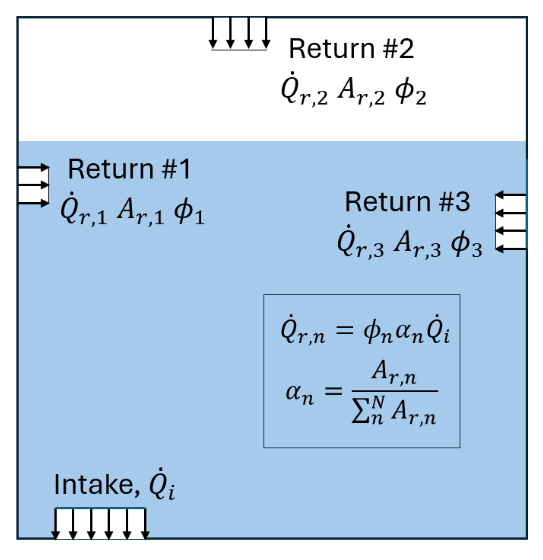
National recirculation system with multiple recirculation returns.

Full Recirculation Proportional Return

For systems with full recirculation and proportional return, \(\dot{Q}_{r,n}(t)\) is a function of \(\dot{Q}_i\) via the inlet area \(A_{r,n}\) and the corresponding inlet area fraction \(α_n\). For a system with a single intake and single return, such that \(n=1\) and \(α=1\), this relationship reduces to \(\dot{Q}_r(t)=\dot{Q}_i(t)\).

Partial Recirculation and Proportional Return

For systems with partial recirculation and proportional return, \(\dot{Q}_{r,n}(t)\) is a function of \(\dot{Q}_i(t)\) via \(A_{r,n}\) as well as a user-set return ratio \(ϕ_n\) for return \(n\). Setting \(ϕ_n\) to a value less than 1 implies that less fluid reenters the system through the recirculation return(s) than exited the system through the recirculation intake. This will cause the fluid volume to decrease over time. For a system with a single intake and single return, such that \(n=1\) and \(α=1\), this relationship reduces to \(\dot{Q}_r(t)=ϕ_r\dot{Q}_i(t)\).

Return Ratio: dimensionless | The ratio of volume flow rate returning through the recirculation return relative to the flow rate expected from the inlet area fraction and intake flow rate (see figure above). A fraction below 1 implies that less fluid reenters the system through the recirculation return(s) than exited the system through the recirculation intake. This setup will cause the overall fluid volume to decrease over time. A fraction above 1 implies that more fluid reenters the system through the recirculation return(s) than exited the system through the recirculation intake. This setup will cause the overall fluid volume to increase over time.

Note

The return ratio only works with Free Surface.

Custom Return Ratio

Fraction of the total intake flow that returns through the associated recirculation inlet. Expression may be a function of the inlet area fraction, \(α_i\), time, and any other system global variables. The realized flow rate through the recirculation inlet will be equal to the total recirculation intake flow rate times the user-specified fraction. This is relevant for systems with non-uniform pressure losses between two or more return lines connected to a single intake.

Recirculation Flow Ratio UDF: dimensionless | This UDF defines the fraction of the total intake flow that returns through the associated recirculation inlet. The realized flow rate through the recirculation inlet will be equal to the total recirculation intake flow rate times this user-specified fraction. This is a System UDF.

Download Sample File: Recirculation Flow Ratio

Recirculation Delay

s | Number of seconds of transit time the recirculation loop presents to particles and scalar fields moving through the recirculation line. This transit delay applies only to particles and scalar fields. Conceptually speaking, this time is related to the length of the return line divided by the average velocity within the line. A value of zero implies fluid leaving the system returns immediately through the recirculation return. This delay is illustrated as part of the model scalar recirculation file.

Target Pressure

Off

On: When this is selected, the Target Pressure Value will launch.
Target Pressure Value: Pa | This represents the target pressure the simulation will attempt to achieve while satisfying the outflow boundary condition. It is recommended for single-phase systems.

Poiseuille¶

A fully developed laminar velocity profile. This parameter imposes the parabolic laminar flow profile for the specified average velocity.

Download Sample File: Poiseuille

Velocity Unit X UDF: unitless | This UDF defines the x-component of the velocity unit vector. Values may be positive or negative. The initial value of the UDF should be zero. This is a System UDF.
Velocity Unit Y UDF: unitless | This UDF defines the y-component of the velocity unit vector. Values may be positive or negative. The initial value of the UDF should be zero. This is a System UDF.
Velocity Unit Z UDF: unitless | This UDF defines the z-component of the velocity unit vector. Values may be positive or negative. The initial value of the UDF should be zero. This is a System UDF
Average Velocity UDF: m/s | This UDF defines the average velocity along the boundary condition surface. For Poiseuille flow through circular pipes, the centerline velocity will be two times this mean value. Positive values move in the direction of the velocity unit vector. Negative values move in the opposite direction of the velocity unit vector. This is a System UDF.

Volume Flow Rate¶

A volumetric flow rate along the boundary condition surface. Value may be time-dependent. The solver converts this to a velocity boundary condition using the calculated area of the inlet.

Download Sample File: Volume Flow Rate

Velocity Unit X UDF: unitless | This UDF defines the x-component of the velocity unit vector. Values may be positive or negative. The initial value of the UDF should be zero. This is a System UDF.
Velocity Unit Y UDF: unitless | This UDF defines the y-component of the velocity unit vector. Values may be positive or negative. The initial value of the UDF should be zero. This is a System UDF.
Velocity Unit Z UDF: unitless | This UDF defines the z-component of the velocity unit vector. Values may be positive or negative. The initial value of the UDF should be zero. This is a System UDF
Volume Flow Rate UDF: m ³ /s | This UDF is an expression for volume flow rate. Positive values move in the direction of the velocity unit vector. The flow rate can be a function of the pressure realized along the boundary condition. Negative values move in the opposite direction of the velocity unit vector. This is a System UDF.

Mass Flow Rate¶

A specified mass flow rate along the boundary condition surface. Value may be time-dependent. The solver converts this to a velocity boundary condition using the calculated area of the inlet and fluid density.

Download Sample File: Mass Flow Rate

Velocity Unit X UDF: unitless | This UDF defines the x-component of the velocity unit vector. Values may be positive or negative. The initial value of the UDF should be zero. This is a System UDF.
Velocity Unit Y UDF: unitless | This UDF defines the y-component of the velocity unit vector. Values may be positive or negative. The initial value of the UDF should be zero. This is a System UDF.
Velocity Unit Z UDF: unitless | This UDF defines the z-component of the velocity unit vector. Values may be positive or negative. The initial value of the UDF should be zero. This is a System UDF
Mass Flow Rate UDF: kg/s | This UDF defines the expression for mass flow rate. Positive values are in the direction of the velocity unit vector, negative value are in the opposite direction. This is a System UDF.

Inlet Single Pulse¶

A single pulse boundary condition with a user-defined start time, flow rate, and duration. The start time is the time at which the boundary is activated. The flow rate can be expressed as either velocity, volumetric flow rate, or mass flow rate.

Download Sample File: Inlet Single Pulse

Velocity Unit X UDF

unitless | This UDF defines the x-component of the velocity unit vector. Values may be positive or negative. The initial value of the UDF should be zero. This is a System UDF.

Velocity Unit Y UDF

unitless | This UDF defines the x-component of the velocity unit vector. Values may be positive or negative. The initial value of the UDF should be zero. This is a System UDF.

Velocity Unit Z UDF

unitless |This UDF defines the x-component of the velocity unit vector. Values may be positive or negative. The initial value of the UDF should be zero. This is a System UDF

Flow Type

This parameter characterizes the boundary condition applied during the pulse.

Velocity: m/s | A scalar quantity describing the velocity magnitude along the boundary condition surface.
Volume Flow Rate: m ³ /s | Volume flow rate with cubic-meters-per-second units. May be an expression as a function of time. Variables t and boundary condition pressures.
Mass Flow Rate: kg/s | Mass flow rate with kilogram-per-second units. May be an expression as a function of time. Variables t and boundary condition pressures.

Flow Magnitude

The magnitude of the velocity, volume flow rate, or mass flow rate during the pulse. The units of this parameter are governed by the flow type.

Start Time

s | The time at which to start the pulse in seconds.

Duration

s | Defines the pulse duration in seconds.

Inlet Multi Pulse¶

A periodic set of pulses with a user-specified velocity, volumetric flow rate, or mass flow rate.

Download Sample File: Inlet Multi Pulse

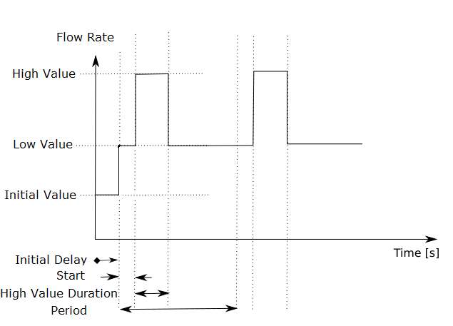
../../../_images/inlet-multi-pulse.png — This Inlet Multi Pulse diagram presents the property grid input variables, as described below.¶

Velocity Unit X UDF

unitless | This UDF defines the x-component of the velocity unit vector. Values may be positive or negative. The initial value of the UDF should be zero. This is a System UDF.

Velocity Unit Y UDF

unitless | This UDF defines the y-component of the velocity unit vector. Values may be positive or negative. The initial value of the UDF should be zero. This is a System UDF.

Velocity Unit Z UDF

unitless | This UDF defines the z-component of the velocity unit vector. Values may be positive or negative. The initial value of the UDF should be zero. This is a System UDF

Flow Type

This parameter characterizes the boundary condition applied during the pulse.

Velocity: m/s | A scalar quantity describing the velocity magnitude along the boundary condition surface.
Volume Flow Rate: m ³ /s | Volume flow rate with cubic-meters-per-second units. May be an expression as a function of time. Variables t and boundary condition pressures.
Mass Flow Rate: kg/s | Mass flow rate with kilograms-per-second units. May be an expression as a function of time. Variables t and boundary condition pressures.

Initial Delay

s | Initial delay time before starting the pulses.

Initial Value

The magnitude of the flow during the initial delay period. The units on this parameter are governed by the user-defined flow type.

Start Time

s | The start time of the high magnitude pulse within the pulse period.

High Value Duration

s | The duration of the high magnitude pulse. During this interval, the flow will assume the high value. Outside this interval, the flow will take the low value.

Period

s | The period of the repeating pulse profile.

High Value

The value of the high magnitude pulse. The units on this parameter are governed by the user-defined flow type.

Low Value

The value of the low pulse. The flow will assume this value outside the duration of the high value. The units on this parameter are governed by the user-defined flow type.

Pump Curve Intake¶

A user-imported pump curve links the flow rate along the boundary condition surface to an instantaneous pressure difference. This difference is calculated by taking the pressure at the pump intake (i.e., along this boundary condition surface) and subtracting the pump discharge pressure.

A pump curve, as illustrated below, is generated experimentally and is available upon request from the pump manufacturer (pump curves tailored to specific fluids and specific pump operating conditions may also be available upon direct request). Most pressure–versus–flow-rate pump curves are generated using a reference fluid (i.e., water) with the pump operating at a reference speed (i.e., 1750 RPM in the figure flow). These results can be extrapolated to other fluid and pump operating speeds.

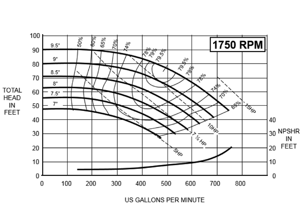
../../../_images/pumpcurve.png — Typical single stage pump curve. Image adapted from Pumps&Systems.¶

The pressure of the pump curve is sometimes characterized as the height of the liquid column. Conceptually speaking, this height represents the pressure head the pump can deliver at a given fluid flow rate. This fluid height must be converted into a fluid pressure (Pascal) when importing the pump curve. The pump discharge at each pressure is typically reported as either a volumetric flow rate (e.g., GPM or m³/hr, etc.) or a mass flow rate (kg/s). When a volumetric flow rate is specified, the discharge rate must be converted to m³/s. When a mass flow rate is specified, the discharge rate must be converted to kg/s.

Download Sample File: Pump Curve Intake

Velocity Unit X UDF

unitless | This UDF defines the x-component of the velocity unit vector. Values may be positive or negative. The initial value of the UDF should be zero. This is a System UDF.

Velocity Unit Y UDF

unitless | This UDF defines the y-component of the velocity unit vector. Values may be positive or negative. The initial value of the UDF should be zero. This is a System UDF.

Velocity Unit Z UDF

unitless | This UDF defines the z-component of the velocity unit vector. Values may be positive or negative. The initial value of the UDF should be zero. This is a System UDF

Pump Curve Units

The units of flow rate of the pump curve. The option selected will be displayed in the Pump Curve Data Table below.

Mass: kg/s | The pump curve flow rate is defined as a mass flow rate.
Volume: m/s | The pump curve flow rate is defined as a volume flow rate.

Pump Curve Data Table

This table pairs specific pressure change values with their corresponding flow rates, effectively forming a characteristic curve for the pump.

The table consists of two equal-length columns: (i) pressure change and (ii) flow rate. The units on the pressure change column are Pascals. The units on flow rate column are either kg/s or m ³ /s, depending on the Pump Curve Units.

At runtime, the solver computes the flow rate along the boundary condition as a function of pressure by interpolating from this data. The flow rate can be based on either volumetric flow rate or mass flow rate. If the curve is specified using a mass flow rate, the user must specify the reference density used by the pump manufacturer to develop the Pump Curve.

The table must contain at least one row but no more than 1000 rows. This is a two-column table.

When the Pump Curve Units are set to Mass, the following selection will launch:

Pump Curve Reference Density: kg/m ³ | The density of the fluid used to define the pumping curve. At runtime, the code will scale the mass flow rate specified in the table by the ratio of the simulation fluid density to this reference density.

Note

For systems with multiple fluids (e.g., two-fluid immiscible systems or miscible systems where fluid density option is on), users should use Volume Pump Curve Units to avoid any ambiguity associated with the reference versus realized fluid densities.

Pump Discharge: This is the boundary condition representing the pump discharge. It is selected from the list of already-defined boundary conditions. The pressure difference between the pump intake and pump discharge informs the fluid flow rate via the pumping curve.

Note

The selected pump discharge boundary condition should have a recirculation boundary condition.