Cooling and Dilution
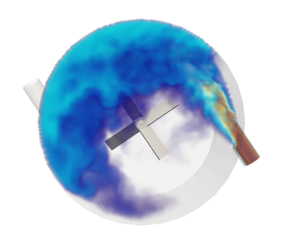
Download Sample File: Cooling and Dilution
Cooling and dilution processes are widely used across real‑world industrial applications to improve the safety and stability of the process environment. They are integral to operations in industries such as chemical and pharmaceutical manufacturing, biotechnology, food and beverage production, medical and laboratory settings. They are equally useful in environmental and utility systems, including wastewater treatment and thermal discharge management.
Key words: cooling, dilution, import external geometry, thermal field, UDF
Introduction
Cooling and dilution combine two essential operations:
Cooling: Removing heat from a substance or system to reduce its temperature
Dilution: Lowering the concentration of a substance by adding a solvent—most commonly water
Each operation serves a distinct purpose. Cooling prevents overheating, equipment damage, and unwanted reaction rates, while also helping maintain product quality and process stability. Dilution reduces reactivity or hazard levels, enables the process to reach a target concentration, and improves dosing accuracy. Both contribute to safer handling of the final mixture.
When combined, cooling and dilution allow simultaneous control of temperature and concentration, improving the safety and stability of the process environment.
The Problem
This guide focuses on modeling a cooling and dilution scenario: high‑temperature acid and cooling water streams are injected into a water‑filled tank. The system must blend the two streams to cool and dilute the acid, making it safe for handling.
We have been asked to evaluate if an existing vessel can be re-purposed to support the cooling and dilution process. The tank design (provided as a .step file) features two inlets entering tangentially on the vessel walls and one outlet pipe entering vertically through the lower head of the vessel. The goal is to predict and understand thermal blending behavior, temperature distributions, acid blend times, concentration distribution, and minimum residence times (to identify potential bypassing) within the tank. These parameters will characterize how the system performs with regard to the cooling and dilution process.
The mixing and dilution system consists of a fully insulated tank equipped with a 0.25 m pitch‑blade impeller (four blades, 45° pitch angle). The impeller is centered on the vertical axis of the tank—positioned with 0.16 m clearance above the tank bottom—and operates at 60 rpm.
Initially, the tank is filled with water at 300 K and features three openings: two side inlets and a bottom outlet. Through the first inlet, acid is introduced at a concentration of 2 mol/L, flowing at 1 m/s and 320 K. This injection begins 5 seconds after the simulation starts, allowing the flow field to develop beforehand. The second inlet supplies water at 1 m/s and 300 K. The bottom outlet is set as a constant pressure boundary at 1 atmosphere, such that flow introduced through the two inlets exits freely and fluid is not accumulated or lost in a non-physical manner.
Define the Problem and the Model Strategy
The first step in solving an engineering problem is to define the problem by identifying what must be modeled, the required outputs, the available inputs, the constraints, and the potential challenges. With these requirements defined, engineers can develop an appropriate modeling strategy, including selecting the physical models, constructing the geometry, and representing the process.
In this case, part of the geometry is supplied as an external file and will be imported as a static body. The impeller will be created using M‑Star’s predefined geometry tools represented by a moving body. The fluid behavior will be represented using a single‑phase model, since the system contains only one liquid phase and all the components are fully miscible, characteristic of the dilution process. The acid will be tracked using a scalar field, and the temperature distribution will be calculated using a thermal field. The inlets and outlet will be defined using static inlet/outlet boundary conditions, the acid injection will be controlled through a user-defined function (UDF), and the outlet will be modeled as a constant pressure outlet boundary condition.
This forms the initial conceptual plan for the simulation—a broad outline of the steps required to build the model, generate the necessary data, and post‑process the results.
The tank geometry has been provided, and it is good practice to review it carefully. Inspecting the file in a CAD tool or importing it into M‑Star Pre allows us to examine its quality, features, and characteristics.
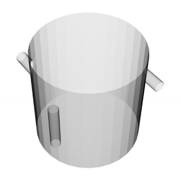
Provided Tank
As we examine the M-Star-supplied geometry, we see that the vessel is asymmetrical. For the purposes of this study, the inlet located closest to the outlet pipe will be used for the acid injection, while the inlet on the opposite side will serve as the water feed.
Build the Simulation
Geometry
To begin building the simulation, we first create the solid components involved in the model: the tank and the impeller. The tank is accessed as an external geometry file, while the impeller will be provided using M‑Star’s predefined components.
We start by creating a solid body to import the tank, select:
Create → Static Body
In the popup window, choose Import from file…, navigate to the location of the tank geometry file (CoolingDiluting.stp), select it, and click Open. The geometry will appear in the Add Geometry window, where you can inspect it, verify its dimensions, and confirm that it is the correct file. Once satisfied, click OK. The tank will then appear in M‑Star Pre as a child geometry of the static body. Rename this Static Body to “Tank”—a good practice that helps maintain clarity, especially in larger assemblies with multiple solid components.
Next, we create the pitch‑blade impeller, select:
Create → Moving Body
In the Add Geometry window, choose:
Parametric → Impeller → Pitch Blade
Click OK, and M‑Star will generate a moving body containing a parametric pitch‑blade impeller. The impeller dimensions and position will be adjusted to better address the intended cooling and dilution service of the system. To reposition, select the Moving Body in the Model Tree, choose Move from the toolbar, and enter 0.185 m in the “Y =” Translation Vector entry field to shift the impeller vertically in the positive Y‑direction. The GUI will show a wireframe representation of the impeller in its future position prior to completion of the operation, allowing confirmation of the intended distance and direction. This places the impeller centerline 0.185 m above the tank bottom and includes an additional 0.025 to account for the height of the mixer impeller.
Check the Moving Body settings and ensure the rotation speed is set to 60 rpm. Then select the child geometry Pitch Blade and verify the diameter, pitch angle, and number of blades. Since this matches the required specifications, no changes are needed except to extend the shaft length to 0.35 m, allowing it to reach the top of the vessel. Rename the moving body to “Impeller”.
Boundary Conditions
Now we define the boundary conditions, beginning with the outlet at the bottom of the tank:
Create → Static Inlet/Outlet
Use the Select Faces selection tool to select the edges that define the outlet. This is the most reliable option for a STEP format solid model. Ensure the direction vector points outward, then click OK. In the boundary condition menu, set the type to Pressure. Adjust the Buffer Length Option to SpecifiedValue and set the buffer length to 0.025 m (50% of the outlet diameter). Rename this boundary condition “Outlet”.
Note
This buffer stabilizes the simulation by locally increasing viscosity adjacent to the outlet boundary region, thereby reducing the likelihood of local flow incompatible with the definition of the boundary. This will have a negligible impact on the representation of the bulk and movement of fluid through the outlet pipe, but it can begin to influence local property values reported at the outlet, such as pressure.
The longer the buffer length, the greater its influence (which can be helpful for stability if an inlet/outlet resides in a region of intensely turbulent flow); but if a buffer equal to the full outlet diameter becomes necessary to maintain stability, the model setup should be reviewed for alternative stabilization strategies.
Next, create the water inlet. Add another Static Inlet/Outlet and select the edges of the pipe opposite the outlet. Ensure the direction points into the tank and click OK. Note that the boundary condition type has defaulted to Velocity (the intended option); confirm that the inlet velocity is aligned with the pipe axis, and set the velocity magnitude to 1 m/s. Enable the Pressure Filter, set it to On, and define a time constant of 8 seconds. This applies a moving average that smooths fluctuations and improves numerical stability. Rename this boundary condition “Inlet_Water”.
Note
As the Lattice Boltzmann representation of fluid has slight numerical compressibility, pressure fluctuations can sometimes arise at inlet and outlet boundary condition cells. The inlet/outlet pressure filter option can be enabled to help eliminate fluctuations at the boundary by temporally smoothing the fluid pressure at the boundary (where a time constant on the scale of a few seconds often behaves well). Additionally, reducing the simulation time step size or extending the ramp period of the inlet/outlet can help avoid such irregular behavior.
Finally, create the acid inlet using the same procedure, selecting the edges of the pipe located closest to the outlet. Ensure it is defined as a velocity inlet and that the velocity vector aligns with the pipe axis. Since the acid injection begins at t = 5 seconds, the velocity magnitude cannot be a constant value. Instead, we will define it using a UDF. Open the Velocity Magnitude UDF editor by selecting the blue icon.
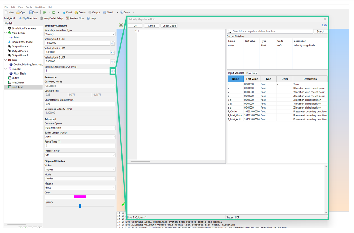
Inlet Velocity UDF
For any time earlier than 5 seconds, the inlet velocity is set to zero. Once the simulation time exceeds 5 seconds, the velocity reaches 1 m/s. To make the model both more realistic and more numerically stable, we introduce a ramp‑up period for the acid injection. Instead of jumping immediately to full velocity, the flow increases gradually over a span of 0.5 seconds. The resulting velocity profile is illustrated in the graph below.
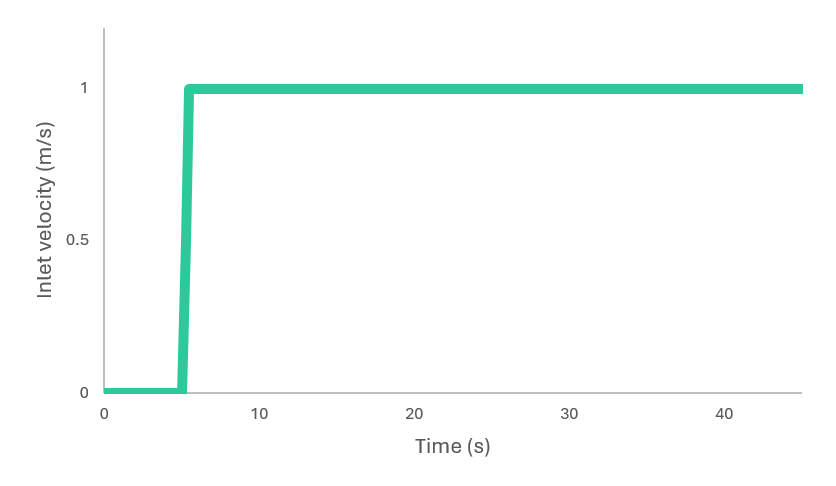
Velocity Profile Acid Inlet
The corresponding UDF can be written as follows:
// Inlet velocity: it is set to 0 for the initial 5 seconds, then it ramps up
// linearly for 0.5 seconds to reach 1 m/s. From that point onward, the
// inlet velocity remains constant at 1 m/s.

float velocity = 1.0;      // Steady inlet velocity [m/s]
float tstart = 5.0;        // Time when the inlet starts working [s]
float rampuptime = 0.5;    // Time over which the velocity increases linearly [s]

if (t < tstart) {
    value = 0;
} else if (t < tstart + rampuptime) {
    value = (velocity / rampuptime) * (t - tstart);
} else {
    value = velocity;
}
Insert this code into the UDF editor and verify its behavior—testing with several time values is always good practice to ensure the logic works correctly and does not produce unintended results. Once the code checks out, click OK to save it.
As with the water inlet, this boundary condition requires a pressure filter to improve numerical stability. Set the Pressure Time Filter Constant to 8 seconds, matching the value used previously, since running the model without this filter produces fluctuations with a period of roughly 5 seconds. Finally, rename this boundary condition “Inlet_Acid.”
Note
It is good practice in any UDF to include a brief description of what the script does, along with clarifying notes wherever needed. It is also helpful to specify the units for every variable declared, as this makes the code easier to understand when the model is revisited later or reviewed by another engineer. Finally, it is important to verify that all units are consistent throughout the script and that the resulting values are expressed in the correct units.
Scalar Field
We use a scalar field to model the acid within the system. No child geometry is required because the acid will be introduced directly through its designated inlet. Create the field by selecting:
Create → Scalar Field
When the Add Geometry window appears, simply click Skip. In the model tree, rename the scalar field to “Acid,” then define its properties. The units should be set to moles, since the provided concentration data is expressed in these units. The diffusion coefficient can remain at its default value, as can the initial background value, because the tank initially contains no suspended acid.
Next, we assign the scalar behavior at each boundary. In the Inlet Outlet Boundary Conditions section of the Scalar feature’s settings, set the scalar boundary condition to Zero Gradient for the Outlet, allowing acid to exit the vessel while assuming downstream disturbances do not influence how the compound leaves the tank. For Inlet_Water, define the scalar as a Specified Value of 0, since no acid enters through this inlet.
Finally, configure the acid behaviour at Inlet_Acid. As with the velocity, this boundary condition will require a UDF. However, the approach differs slightly: here we specify the volumetric concentration (mol/L) rather than a velocity profile. Because the concentration is tied to the inlet flow rate, no ramp‑up is required. We only need to define when the injection begins and the concentration value. The UDF is therefore:
// Acid injection: define the feed concentration and when the feed becomes
// active. No acid is injected during the initial 5 seconds. After that,
// acid is injected at a constant concentration of 2 mol/L.

float acid_concentration = 2.0;   // Acid concentration at the inlet [mol/L]
float tstart = 5.0;               // Time when acid injection begins [s]

if (t < tstart) {
    value = 0;
} else {
    value = acid_concentration;
}
After inserting the code, perform the necessary checks to ensure it behaves as expected, then click OK to save it.
Note
A scalar concentration could simply be entered as a constant and applied to the boundary condition region throughout the simulation. However, this would assign the specified concentration to the inlet boundary cells before the inlet volume flow is initiated, allowing a small quantity of scalar to diffuse into the domain before the intended injection occurs. For short time periods, this is negligible, but for large inlet boundaries or extended delays it could be significant.
All remaining scalar field parameters for the “Acid” field can remain at their default values. Once completed, the “Acid” scalar field will appear as shown below.
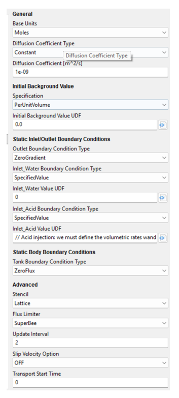
Acid Scalar Field Parameters
Thermal Field
The next step in setting up the model is to create the thermal field, which allows us to compute local temperature, heat transfer, and related thermal effects. To enable the thermal field in M‑Star CFD, create a new component by selecting:
Create → Thermal
A new branch called Thermal Field will appear in the Model Tree; select it to adjust the settings.
The thermal properties can maintain their default values, as these correspond to water—the bulk fluid in the tank. The initial conditions at t = 0 are also constant, since the tank is initially filled with water at 300 K. The minimum and maximum temperature limits can be left at their default values; these inform the solver of the expected temperature range in this system. Dissipation Heating remains enabled, Global Heating is set to 0, and Local Heating stays disabled, matching the default configuration.
For the boundary conditions, the outlet is assigned a Zero Gradient condition, following the same reasoning used for the scalar field. The water inlet is set to a constant temperature of 300 K, as water enters continuously at this temperature from the start of the simulation.
For Inlet_Acid, we again use a UDF. The high‑temperature fluid entering through this inlet is the acid, and until injection begins, no thermal contribution should be applied. The UDF follows a similar structure to the velocity UDF but for a different physical reason: we introduce a linear temperature ramp to represent the acid cooling slightly while stationary in the pipe before injection. Thus, the acid initially enters at 300 K, and its temperature increases linearly over 2 seconds until it reaches its full injection temperature of 320 K. The UDF is:
// Acid injection temperature: before acid injection begins, the inlet
// temperature is equal to the initial bulk fluid temperature (300 K).
// It is assumed that the acid cools slightly while waiting to be injected,
// and that it takes 2 seconds for the inlet temperature to increase
// linearly to the target acid injection temperature of 320 K.

float initial_bulk_temperature = 300.0;   // Initial temperature in the tank [K]
float acid_temperature = 320.0;           // Acid injection temperature [K]
float tstart = 5.0;                       // Time when acid injection begins [s]
float rampuptime = 2.0;                   // Time for the temperature to increase linearly [s]

if (t < tstart) {
    value = initial_bulk_temperature;
} else if (t < tstart + rampuptime) {
    value = initial_bulk_temperature
          + ((acid_temperature - initial_bulk_temperature) / rampuptime)
          * (t - tstart);
} else {
    value = acid_temperature;
}
For the tank walls, the boundary condition remains adiabatic, as specified in the problem statement—we assume no heat is exchanged through the insulation of the vessel walls. All remaining thermal parameters can be left at their default values. An illustration of the final configuration is shown below.
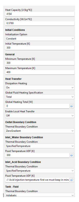
Thermal Field Parameters
Final Checks
At this stage, the model includes all required physics, but a few important verifications and adjustments remain. First, we will review the fluid setup in the Model Tree. Since this is a single‑phase system with water as the bulk fluid, we will open the Single Phase Model settings and confirm in the Property Grid that the default properties match those of water—which they do. Returning to the Model Tree, on the Main Lattice branch we will ensure that the fill point lies inside the tank volume rather than on a wall, tank internal, or moving body geometry.
Next, we will adjust the simulation parameters. The total simulation time is increased to 90 seconds to allow the solution to evolve toward a stable state. We must also consider the spatial and temporal resolution. As discussed earlier, it is always recommended to perform a sensitivity study when running a new simulation to ensure that results are not influenced by discretization choices. In this case, a separate study has already been completed, showing that 175 elements across the tank diameter and a Courant number of 0.01 provide a sufficiently accurate, discretization‑independent solution.
Define Output
With the model prepared, we now consider the outputs we want to generate. M‑Star provides a wide range of default outputs, including 2D slices, 3D volumes, and tabular data. For this case, we will adjust some of the output planes to improve clarity during post‑processing.
Output planes are particularly useful for visualizing the 3D flow field and associated quantities in a lightweight format. By default, M‑Star creates three planes—one perpendicular to each Cartesian direction—positioned at the geometric center. While the default X‑ and Z‑planes are suitable, the default Y‑plane lies in the middle of the tank, which is not ideal for this analysis. Instead, we will reposition it to align with the impeller and create an additional y‑plane aligned with the inlets.
In the Model Tree, select Output Y Plane and set the Intercept Value to 0.185, placing it at the impeller height. Rename it “Output Plane Y_Impeller.” Then create a new output plane:
Create → Output plane
Set the Axis Direction to Y, and assign an Intercept Value of 0.375, positioning it at the inlet level. Rename this plane “Output Plane Y_Inlets.”
Next, open the Output settings. In the window that appears, reduce the Statistics Write Interval to 0.005, and set the Planes/Probes Write Interval to 0.05. You may enable any additional quantities you wish to access during post‑processing, though for this case we will keep the default selections. In the Volume tab, change the output interval to 0.5, and in the Static Bodies tab, enable Fluid Temperature. Once all settings are adjusted, click OK to confirm.
With everything configured, select Solve and run the simulation.
This video of the simulation highlights the scalar acid concentration, the volume temperature, and the fluid streamlines. Although the impeller appears stationary, it is in fact rotating—this is a stroboscopic effect caused by a sychronization of the frame rate and impeller speed.
Post-Process and Analyze the Results
As the simulation begins, the impeller immediately drives the bulk fluid downward while water enters the vessel at 300 K at 1 m/s. After the first 5 seconds, the acid injection starts, entering at a concentration of 2 mol/L, a temperature of 320 K, and a velocity of 1 m/s. To understand how the system evolves once both streams are active, we examine the velocity field, the acid concentration, and the temperature throughout the entire tank volume. Different scales and color maps are used to make the internal flow structures and mixing behavior as clear as possible.
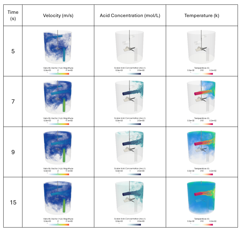
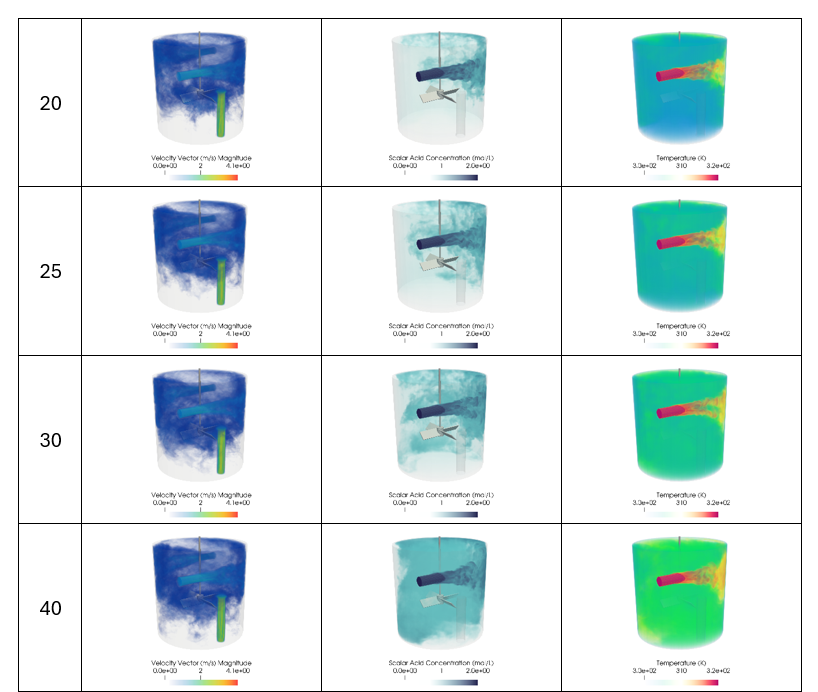
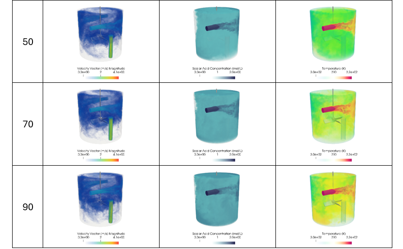
The acid jet strikes the opposite tank wall and then begins to turn, spreading across the upper region of the vessel. During the first ten seconds of the simulation, this creates a clear division in the tank: the upper section becomes enriched with acid, while the lower region remains at much lower concentrations. The temperature field follows the same pattern, with pronounced thermal gradients developing between the top and bottom of the vessel. As the simulation progresses, the impeller gradually breaks down these divisions. Its circulation pulls the acid‑rich fluid downward, increasing the concentration in the lower region, and the temperature is transported in a similar manner. By the end of the run, the bulk fluid shows a nearly uniform distribution of both acid concentration and temperature.
The dominant flow mechanisms in the tank can be understood by dividing the vessel into two zones. Above the impeller, the motion is governed primarily by the incoming jets, which drive strong directional flow and lead to significant gradients in both temperature and species concentration near the top of the tank. Below the impeller, however, the rotating blades homogenize the fluid, smoothing out variations in both thermal and concentration fields.
With this behavior in mind, the key question becomes clear: Is the mixture leaving the tank sufficiently diluted? To answer this, we examine the acid concentration at the outlet.
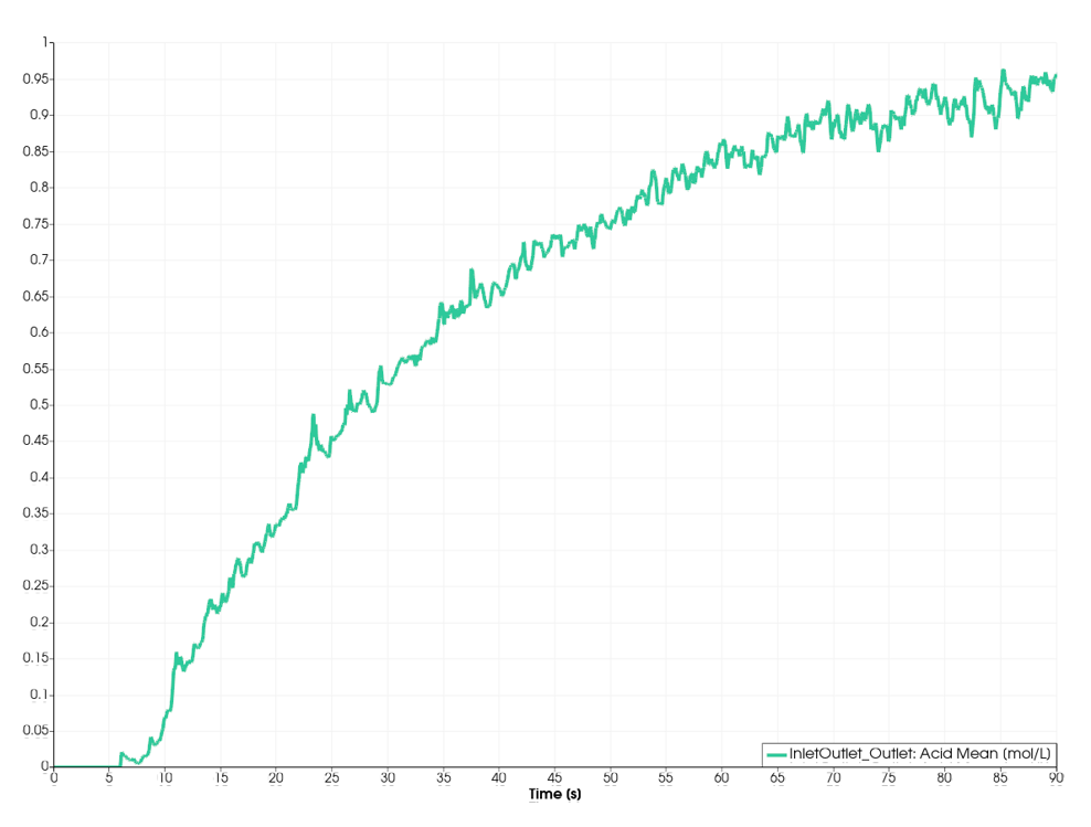
Time evolution of acid concentration on outlet
The graph shows that the acid concentration at the outlet increases over time following a first‑order exponential trend. From around 75 seconds onward—approximately 70 seconds after the acid injection begins—the curve levels off, indicating that the bulk concentration has stabilized and a steady state operating condition has been reached. This stabilization does not necessarily confirm that the fluid leaving the tank is well mixed, however. A statistic measure of the consistency of the outlet boundary might be considered to qualify if the vessel contents are sufficiently uniform to satisfy the required dilution process result. Once steady operating conditions have been reached, the variance or coefficient of variation of the outlet concentration provides a measure of uniformity at the outlet. Users can use this metric to assess whether fluctuations are sufficiently small for downstream operations, such as filling or dispensing, to produce a consistent product. Although outlet statistics are useful for assessing product consistency, they should be considered alongside other mixing diagnostics to evaluate the degree of mixing throughout the vessel.
The plot also highlights that no acid appears at the outlet during the first 5 seconds, as expected. Using this information, we can estimate the minimum residence time. The first detectable trace of acid scalar occurs at 6.05 seconds, meaning this is the earliest moment acid exits the tank. Since injection starts precisely at t = 5 seconds, the minimum residence time is 1.05 seconds.
Finally, we assess the temperature distribution within the vessel. By plotting the temperature field at the final simulation time, we can visualize how heat has accumulated and dispersed throughout the tank. In addition, examining the average temperature over the full simulation provides a clear picture of its overall evolution.
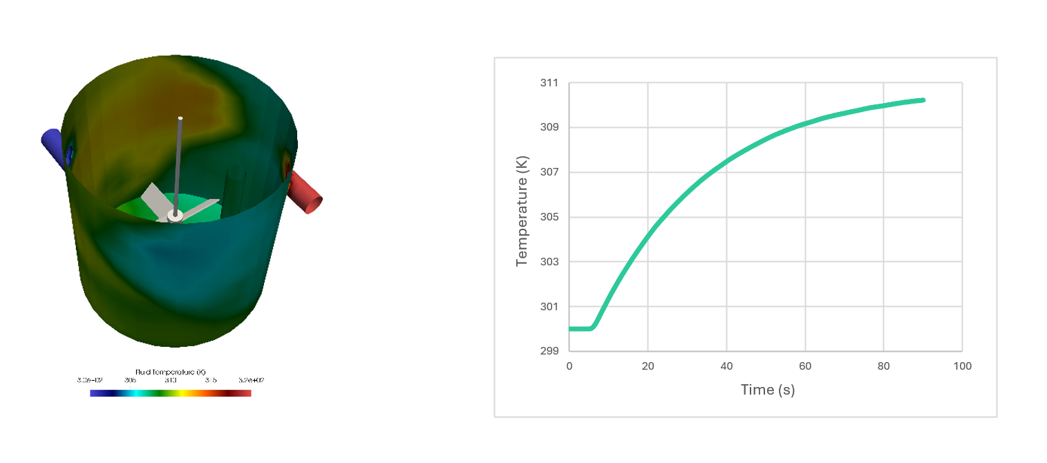
Temperature map on tank surface (at t=90 seconds) and Temperature evolution on the system
Examining the temperature evolution, we see the system gradually settling toward an equilibrium of roughly 310 K. This behavior is entirely consistent with the operating conditions: the tank receives two streams of equal flow rate, one at 300 K and the other at 320 K, so after an initial transient—during which the bulk fluid warms rapidly from its initial 300 K—the temperature converges toward the expected midpoint.
However, despite this overall trend, the temperature field inside the vessel is far from uniform. The final temperature distribution reveals pronounced gradients across the tank. The highest temperatures appear in the acid‑injection pipe and in the regions of the tank wall directly impacted by the incoming jets. In contrast, the lower part of the vessel, dominated by the impeller’s circulation, shows a more homogenized thermal field. The outlet pipe temperature, visible in the final snapshot, stabilizes at approximately 310 K, matching the bulk equilibrium value. Variations in outlet temperature can be considered analogously to the acid concentration.
In summary, the provided tank and agitator design produces a relatively well‑mixed outlet stream in which the mean acid concentration and temperature leaves the vessel with CoV of X%. Equilibration of the transient continuous system between discrete operating conditions requires roughly 70 seconds from, in this case, the moment acid injection begins. It is also important to note that, although the outlet stream is well mixed, the internal mixing is not perfectly homogeneous, and there is still variance in the properties of the effluent. Significant spatial temperature and concentration gradients necessarily persist throughout the vessel.