Fluid Interface

The Fluid Interface control panel specifies which field quantities are calculated and exported along the fluid interface. The fluid interface is a two-dimensional surface that represents the boundary between regions of differing phase or composition within the computational domain.

For free-surface simulations, the interface separates the liquid phase from the empty headspace. For immiscible two-fluid simulations, the interface represents the surface separating the two fluid phases. These outputs retain coordinate information associated with each field value along the interface, rather than reporting single-valued reduced outputs.

The position of the interface within the transition region is defined by a volume-of-fluid (VOF) isosurface contour, corresponding to a specified volume-fraction value. In addition to the primary interface, the solver can identify and extract discrete, disconnected interface regions, enabling detection and tracking of individual satellite structures of a selected fluid phase

Interface data are written to binary .vtp files for visualization, animation, and analysis within M-Star Post or any compatible VTI file reader. These files are printed at both the Plane/Probe Write Interval as well as the Volume Write Interval. This makes the output frame-consistent for visualization and animation in both 2D and 3D renderings. The names of these two sets of output files are Slice VOF Surface and Volume VOF Surface, respectively.

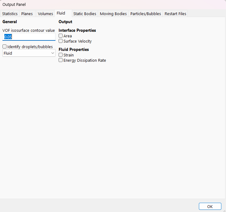
Output Panel

General

VOF Interface Value

The VOF interface value represents the specific threshold used to visualize and track the sharp interface between two immiscible fluids. Because the phase fraction is a scalar field ranging from 0 (Fluid 2) to 1 (Fluid 1), an isosurface value of 0.5 is most commonly chosen as the “cut-off” to define the physical boundary, and it is the default value. This value ensures that the interface is positioned where the cell is exactly half-filled with each phase, providing a balanced geometric representation of the surface.

Note

This setting exclusively controls the threshold for graphical rendering and does not influence the underlying physics. Regardless of the value selected for visualization, the solver maintains a fixed isosurface value of 0.5 for any interface reductions, surface tension calculations, and interfacial heat/mass transfer processes.

Identify VOF Structures

When enabled, the solver will identify each separate isolated VOF structure for the selected fluid. The user selects the fluid from the dropdown box. This feature is used to identify discrete/disconnected VOF regions, enabling detection and tracking of individual satellite structures of a selected fluid phase.

Output Control

Local Interface

These properties define fluid properties printed along the free surface.

Local Interface Properties

▢ Velocity Vector

m/s | This defines the three-dimensional fluid velocity vector, \(\vec{V}\), defined as

\[\vec{V}={v_x}\vec{i}+{v_y}\vec{j}+{v_z}\vec{k},\]

where \(v_x\), \(v_y\), and \(v_z\) are the x-, y-, and z-components of the velocity field.

▢ Resolved Strain Rate

1/s | The resolved fluid strain rate is a scalar quantity computed as

\[\dot{\gamma} = \sqrt{S_{ij} S_{ij}},\]

where \(S_{ij}\) is the resolved strain-rate tensor. This corresponds to the magnitude of the strain-rate tensor based on the Frobenius norm.

▢ Energy Dissipation Rate

W/kg | The energy dissipation rate is the rate at which kinetic energy is converted into thermal energy by viscous stresses. The local dissipation rate per unit mass is

\[\epsilon = 2\nu\, \mathbf{S}\!:\!\mathbf{S},\]

where \(\varepsilon\) is the local kinematic viscosity, and \(\mathbf{S}\) is the local strain-rate tensor. The strain-rate tensors used to evaluate the local dissipation rate are evaluated directly from the LBM distribution function. This approach yields a more accurate evaluation of the Frobenius inner product.

▢ {Voxel Variable}

This describes the local magnitude of the Voxel Variable. The selection name is the Dynamic Name of the associated voxel variable.

If VOF Structures is enabled, the following output properties will launch:

VOF Structures

When the Identify VOF Structures option is enabled, the solver automatically identifies and extracts discrete, disconnected VOF structures corresponding to the selected phase. Data associated with each identified structure are written to a new particle set named VOF Structures.

The example below illustrates a globular dispersion regime in which a low-density oil layer is entrained by an agitated impeller into an underlying higher-density water phase. The oil is transported as large, coherent structures, with limited breakup and minimal fine-scale mixing. The left images show the time evolution of the VOF surface, highlighting the contours of the entrained structures. The right images show the individual satellite structures identified by the algorithm.

EXAMPLE

Note

Only VOF structures with a characteristic diameter of approximately six lattice points or larger can be resolved and identified. Structures smaller than this resolution limit cannot be reliably captured using a VOF formulation. For systems that form sub-grid droplets or bubbles, a free surface VOF-to-particle conversion approach should be used. This conversion is available for both Free Surface and Two Fluid immiscible configurations.

For each identified structure, a single particle is created in the VOF Structures particle set. The particle location corresponds to the center of mass of the associated satellite structure.

In addition to position, the following reduced droplet properties associated with each identified droplet or bubble are attached to the corresponding particle in the VOF Structures particle set.

▢ Surface Area

\(m^2\) | This describes the surface area the interface. This area is calculated at VOF isosurface contour value.

▢ Volume

\(m^3\) | This describes the volume contained within the identified VOF structure. The volume is bounded by the VOF isosurface contour value.

▢ Energy Dissipation Rate

W/kg | This includes both resolved and unresolved components near the surface of a droplet or bubble. The identified VOF structure typically spans multiple fluid cells. The Energy Dissipation Rate is the spatial mean of the Energy Dissipation Rate near the droplet or bubble surface.

▢ Adjacent to Wall

This will take a value of 1 when the droplet/bubble is adjacent to a wall and 0 when it is not.

▢ Sauter Mean Diameter

m | The Sauter Mean Diameter is the ratio of the total volume to the total surface area of the droplet or bubble.

\[d_{32} = \frac{6 \cdot V_{\text{bubble}}}{A_{\text{bubble}}}\]

When the droplet or bubble is a sphere, this reduces to the diameter of the sphere. For oblong spheroids or other non-spherical shapes, this diameter is less than a volume-equivalent sphere.

▢ Sphere Diameter

m | The sphere diameter is the diameter of a sphere with equivalent volume.

\[d_{\text{sphere}} = \left(\frac{3 \cdot V_{\text{bubble}}}{4 \cdot \pi}\right)^{1/3}\]

▢ Velocity

m/s | The identified VOF structure typically spans multiple fluid cells. When using the Free Surface model, the velocity is defined as the spatial mean of the fluid velocity near the droplet or bubble surface. When using the Immiscible Two-Fluid model, the velocity is defined as the spatial mean of the selected fluid within the identified structure.