External Accelerations

These are applied on a voxel-by-voxel and particle-by-particle basis. The acceleration vector is a function of the applied motion type. This is superimposed on the gravity vector.

External accelerations are useful for modeling things like shaker tables, sloshing systems, rocking systems, etc.

The dynamics realized using external accelerations are like those that are realized using fluid vessels modeled as moving bodies (with voxelated walls to conserve fluid volume). The differences between the two approaches are (i) the memory requirements and (ii) how accelerations are imparted to the fluid. These points will be discussed in the forthcoming External Accelerations How-to Guide.

When external accelerations are present, the Enable Lab Frame icon becomes available in M-Star Post. Pressing this icon allows user to toggle between reference frames when visualizing the flow.

None

No external accelerations beyond the gravity vector.

Linear Shake

One-dimensional rigid body oscillatory shaking along a set axis with a user-defined motion amplitude and speed. The key features defining this motion type are illustrated in the figure below.

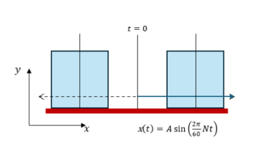
The linear oscillatory shaking can occur along either the X, Y, or Z axis (as defined by the global basis). The linear motion is defined by a Linear Shake Amplitude A and a Linear Shake speed. In the example above, the motion occurs in the x-direction.

Download Sample File: Linear Shake

Linear Shake Direction

This defines the orbit plane (as defined by the global basis). The orbit motion occurs in this orbit plane.

X

This selects the X orbit plane.

Y

This selects the Y orbit plane.

Z

This selects the Z orbit plane.

Linear Shake Amplitude

meters | This parameter defines the amplitude of the shake motion. The stroke is twice the shake amplitude radius.

Linear Shake Speed

rpm | This parameter defines the shaking speed of the table. It characterizes the time required to perform a complete oscillation.

Orbital Shake

Two-dimensional rigid body orbital motion in a set orbital shake plane with a user-defined shake ampliated and shaking frequency. The key features defining this motion type are illustrated in the figure below.

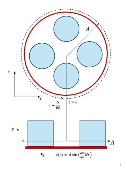
The orbital shake motion can occupy either the XY, YZ, or XZ plane (as defined by the global basis). The orbital motion is defined by an orbital shake amplitude and an orbital shake speed. In the example above, the motion occupies the XZ Plane.

Download Sample File: Orbital Shake

Orbital Shake Plane

This defines the orbit plane (as defined by the global basis). The orbit motion occurs in this orbit plane.

XY

This selects the XY orbit plane.

YZ

This selects the YZ orbit plane.

XZ

This selects the XZ orbit plane.

Orbital Shake Amplitude

meters | This parameter defines the radius of the orbital shake circle. The orbit diameter is twice this orbit radius.

Orbital Shake Speed

rpm | This parameter defines the shaking speed of the table. It characterizes the time required to perform a complete revolution.

Rocking

One-dimensional rigid body rocking about a user-defined axis/pivot point with a user-defined maximum tilt angle and rocking frequency. The key features defining this motion type are illustrated in the figure below.

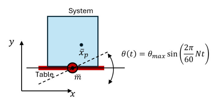
The rocking axis can point in either X, Y, or Z directions (as defined by the global basis) The mount point of the rocking axis is defined by \(m\). The rocking motion is defined by and maximum tilt angle \(θ_{max}\) and a rocking frequency. In the example above, rocking occurs about the Z-axis with a mount point centered on the rocker table.

Download Sample File: Rocking Table

Rocking Axis

This selection defines the axis of rotation.

X

This selects the X-direction of the global basis set.

Y

This selects the Y-direction of the global basis set.

Z

This selects the Z-direction of the global basis set.

Rocking Tilt Angle

degrees | This defines \(θ_{max}\), the maximum tilt angle.

Rocking Speed

rpm | The rocking speed.

Rotation Axis Mount

The location of the rotation axis, \(m\). This is defined relative to the global basis. Since the rocking axis is assumed to be infinitely long, its position along its own direction is irrelevant—-only the two perpendicular coordinates of the mount point matter.

Ball Joint

Three-dimensional ball/socket joint motion. This functionality is useful for describing multi-directional articulation. The key features defining this motion type are illustrated in the figure below. The accelerations from this motion are superimposed on the gravitational acceleration.

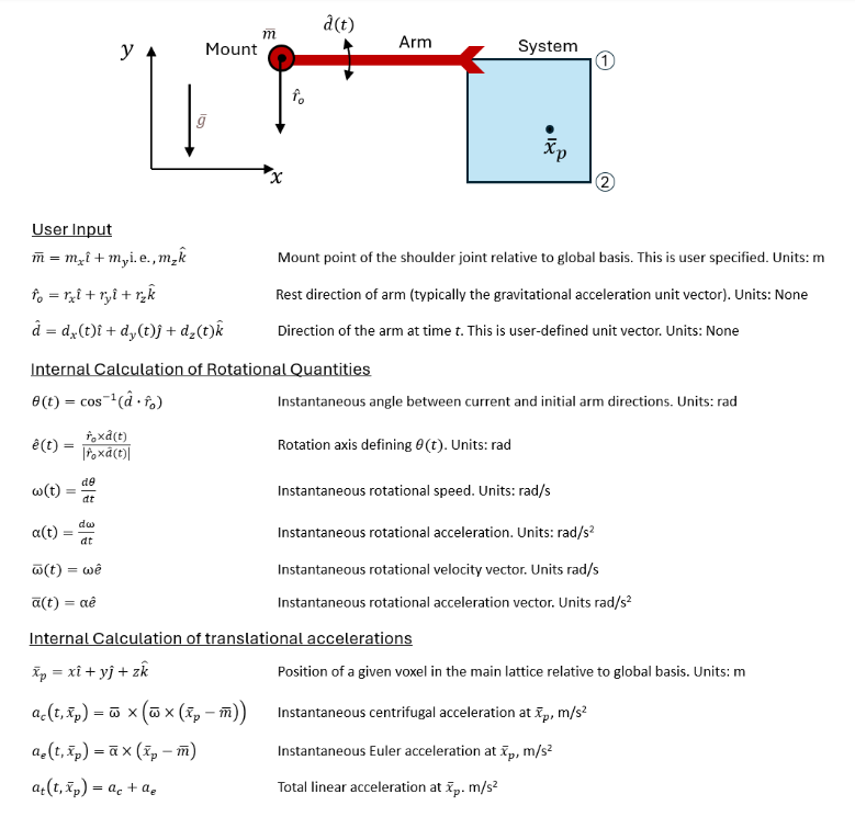
The mount point of the arm, \(\overline{m}\), is the position of the ball joint socket. The direction of the arm at time \(t\), \(\hat{d}(t)\), is a unit vector that defines the instantaneous orientation of the arm. The rest direction, \(\hat{r}_o\), is a unit vector that defines the position of the arm when at rest. This rest vector is typically equal to the direction of gravitational acceleration. Note that all vectors are defined with respect to the global basis set.

The ball joint acceleration is more complex than the other motion types and mandates a bit more discussion. At runtime, per the instructions below, the solver uses input quantities to compute the instantaneous rotational velocity \(\overline{\omega}(t)\) vector and instantaneous rotational acceleration \(\overline{\alpha}(t)\) vector. These rotational vectors are used to calculate the centrifugal acceleration \(a_c\) and Euler acceleration \(a_e\) at each lattice point (using the voxel position relative to the mount point). The sum of these accelerations defines the total acceleration at each point, \(a_t\). The spatial orientations and rotations are represented using quaternions. Note that the rotation axis \(\hat{e}(t)\) is only evaluated when \(|\hat{r}_o \times \hat{d}(t)|\) is non-zero, implying a finite rotation angle.

This requires a UDF which defines the orientation of a three-dimensional unit vector with the arm connected to the ball joint. The unit vector, which is used to indicate a direction, is always dimensionless and always normalized to have a length of 1.0. Individual UDFs are defined for the x, y, and z components of the vector. This vector is defined with respect to the system basis vectors. The time-evolution of this unit vector describes the motion of the ball joint arm.

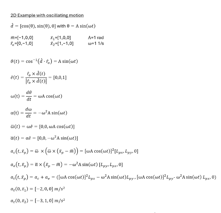
To illustrate the behavior of this system, consider a notional 2D example with oscillating ball joint motion. With this example outlined below, we define the ball joint axis as \(\hat{d} = [\cos(\theta), \sin(\theta), 0]\), where \(\theta = A \sin(\omega t)\), and where \(A\) is 1 rad and \(\omega\) is 1 rad/second. We define the mount point, \(\overline{m}\), to be \([-1,0,0]\) and the arm rest axis \(\hat{r}_o\) to be \([0,-1,0]\).

For illustration purposes, we calculate the total acceleration \(a_t\) at \(t=0\) for two points in the system: Point 1 at position \([1,0,0]\) and Point 2 at position \([1,-1,0]\). Both these points are illustrated in the figure. The corresponding accelerations at these points are \(a_t(0, \overline{x}_1) = [-2, 0, 0] \text{ m/s}^2\) and \(a_t(0, \overline{x}_2) = [-3, 1, 0] \text{ m/s}^2\). More complex three-dimensional motions will produce a more complex acceleration profile.

The implementation of this simple 2D motion is presented below in the example video and file. The arm of the ball joint was added to the system geometry to help illustrate the motion of the cylinder. The ball joint point remains fixed throughout the simulation, while the dynamics of the arm are oscillating about the specified rotation axis. The acceleration, combined with gravity, informs the dynamics of the free surface.

Download Sample File: Ball Joint Unit Vector

Ball Joint Mount

m | Ball joint mount point, relative to the global basis.

Ball Joint Ref Axis

Unit vector describing the reference axis of the ball joint arm. In most cases, this vector is the same as the initial orientation of the ball joint arm. In some advanced cases, this reference axis can be manipulated to modify the initial position of the lattice relative to the ball joint arm.

Ball Joint Unit Vector X UDF

unitless | This UDF describes the time evolution of the X-component of the ball joint unit vector. This is a System UDF.

Ball Joint Unit Vector Y UDF

unitless | This UDF describes the time evolution of the Y-component of the ball joint unit vector. This is a System UDF.

Ball Joint Unit Vector Z UDF

unitless | This UDF describes the time evolution of the Z-component of the ball joint unit vector. This is a System UDF.

Download Sample File: Ball Joint Unit Vector - Shaker Table

The above example demonstrates the External Acceleration > Ball Joint feature for modeling a generic shaker table with four beakers. The shaker table’s motion is controlled independently for rotation about the x-axis (pitch) and y-axis (roll).

In the provided sample file, pitch and roll angle and frequency parameters are defined as Global Constants. Massless tracer particles are used to visualize the flow within each beaker.

Custom Rotation

Custom-defined rigid body rotation, expressed at a time-evolving rotational speed about a fixed rotation axis. The time-evolution of the rotation speed (specified in rpm) is defined using a System UDF. This functionality is useful for modeling systems with time-varying rigid body rotation, such as spinning drums and centrifuge separators. The accelerations from this motion are superimposed on the gravitational acceleration.

Rotation Axis

This unit vector represents the direction of the rotation axis. The three fields define the X, Y, and Z components of the axis vector. These vectors are aligned with the basis X, Y, and Z unit vectors.

Rotation Axis Mount

This point defines the root of the rotation axis. The three fields define the X, Y, and Z position of the root. This position is defined relative to the global basis.

Rotation Speed UDF

rpm | This UDF defines the time-evolution of the rotational speed about the (fixed) rotation axis. Values may be positive or negative. The direction of rotation is indicated by the arrow drawn around the rotation axis in the viewing panel. This is a System UDF.

Download Sample File: Rotation Speed

Custom Translation

Custom-defined rigid body translation, expressed as a time-evolving acceleration in the X, Y, and Z directions. The magnitude and direction of acceleration in each direction is defined using a System UDF. This functionality is useful for modeling systems with time-varying linear accelerations, such as fluid sloshing in trucks, trains, transport vessels, and spacecrafts. The accelerations from this motion are superimposed on the gravitational acceleration.

Download Sample File: Custom Translation Acceleration UDF

Initial Velocity

This is the initial translational velocity vector of the lattice domain. The three fields define the X, Y, and Z components of the velocity vector. These vectors are aligned with the basis X, Y, and Z unit vectors within the system.

Acceleration X UDF

m/s ² | Time-evolution of the lattice acceleration in the X-direction. This is a System UDF.

Acceleration Y UDF

m/s ² | Time-evolution of the lattice acceleration in the Y-direction. This is a System UDF.

Acceleration Z UDF

m/s ² | Time-evolution of the lattice acceleration in the Z-direction. This is a System UDF.