Static Inlet/Outlet Boundary Conditions
Applicability

Overview
There are four options for defining scalar field inlet and outlet boundary conditions. These parameters control the scalar boundary conditions along the boundary condition surface. Each boundary condition can vary in time. Some boundary conditions can vary along the boundary condition surface, as discussed on a case-by-case basis below.
Other boundary conditions are defined separately with their respective families, including fluid, miscible scalar, free surface volume fraction, immiscible two fluid volume fraction, thermal, and particle boundary conditions.
The behavior of these boundary conditions is discussed below, and examples illustrating their workflow are presented on the last section of this page.
{Static Inlet/Outlet} Boundary Condition Type
This parameter defines what scalar field values or fluxes will be applied at each static inlet or outlet. Boundary conditions for inlets and outlets are defined along two-dimensional surfaces. For each scalar field, users can enforce either a Dirichlet or Neumann boundary condition along the surface. A Dirichlet boundary condition defines a set scalar field value along the surface. A Neumann boundary condition defines the scalar field gradient normal to the surface. Scalar field boundary conditions can also be linked to model recirculating systems using a modified form of the Dirichlet boundary condition. This selection has a dynamic name that is linked to the name of the component in the model tree.
Specified Value
A specified value is the Dirichlet boundary condition, which is a fixed value. This type is typically used to specify the species concentration of the fluid entering the system at a given inlet. The set value can be a UDF, written in terms of position, time, and system global variables. This boundary condition is illustrated below in Examples 1 and 2.
- {Inlet/Outlet} Value UDF
base units /L | This UDF defines the species concentration along the boundary condition surface. This value may be an expression of the form f (x,y,z,t), where f>=0, and where x,y,z are relative to the inlet seed point and in the SI unit system. The units are determined by the scalar field background specification type. A value field is added for each boundary condition, identified by the user-set boundary condition name. This selection has a dynamic name that is linked to the name of the component in the model tree. This is a System UDF.
Download Sample File: {Inlet/Outlet} Value
Zero Gradient
A zero gradient boundary condition will match the local species concentration along the boundary condition surface to the local species concentration in the adjacent fluid. This boundary condition type is typically applied at fluid outlets. This is a passive boundary condition, meaning the value is not set by the user but is informed by the upstream flow field and the concentration incoming to the boundary condition surface. The concentration realized at the zero gradient boundary condition will evolve in space and time in response to upstream injection, reaction, and mixing characteristics. This boundary condition is illustrated below in Examples 1 and 2.
Zero Flux
In a zero flux, no species will cross the boundary condition surface. This feature can be used to model semipermeable membranes, which selectively forbid some species from entering/exiting through the boundary condition surface. Interactions with the boundary condition surface will not add/remove species from the system.
Recirculation
Recirculation is used to model recirculation loops and to connect species flux exiting the system via one outlet to species reentering via one or more inlets. This functionality is particularly useful when modeling filtration systems, jet mixing systems, dilution processes, etc. This boundary condition is illustrated below in Example 3.
- {Static Inlet/Outlet} Recirculation Configuration
This configuration defines the coupling between the scalar flow rate reentering the system via the recirculation return boundary condition(s) and the scalar flow rate exiting the system via the associated intake. This selection has a dynamic name that is linked to the name of the component in the model tree. As discussed in the Recirculation Return boundary conditions setup form, the fluid boundary condition along the intake is typically defined as a volume flow boundary with a user-set flow rate of \(\dot{Q}_i(t)\), which is then calculated at runtime from:
\[\dot{m}_i(t)=c_i(t)\dot{Q}_i(t).\]where \(c_i(t)\) is the time-evolution scalar field concentration at the intake. The units on \(c_i\) are defined by the scalar field Base Unit.
Three configuration options are available for defining the return scalar flow rate \(\dot{m}_r,_n\): (i) full scalar recirculation proportional return, (ii) partial scalar recirculation and proportional return, and (iii) custom scalar return ratio.
- Full Recirculation Proportional Return
For systems with full scalar recirculation and proportional return, \(\dot{m}_r,_n\) is a function of \(\dot{m}_i\) via corresponding inlet area fraction \(\alpha_n\). This relationship is illustrated in the figure below. For a system with a single intake and single return, such that \(n=1\) and \(\alpha=1\), this relationship reduces to \(\dot{m}_r(t)=\dot{m}_i(t)\).
- Partial Recirculation and Proportional Return
For systems with partial recirculation and proportional return, \(\dot{m}_n\) is a function of \(\dot{m}_i(t)\) via inlet area fraction \(\alpha_n\) as well as a user-set return ratio \(\phi_n\). For a system with a single intake and single return, such that \(n=1\) and \(\alpha=1\), this relationship reduces to \(\dot{m}_r(t)=\phi_n\dot{m}_i(t)\). Setting \(\phi_n\) to a value less than one implies that less scalar reenters the system through the recirculation return(s) than exited the system through the recirculation intake. This will cause the amount of scalar within the system to decrease over time.
- {Static Inlet/Outlet} Return Ratio
dimensionless | The ratio of the scalar flow rate returning through the recirculation return relative to the scalar flow rate expected from the inlet area fraction and intake scalar flow rate. A fraction below one implies that less scalar reenters the system through the recirculation return(s) than exited the system through the recirculation intake. This setup will cause the overall amount of scalar to decrease over time. A fraction above one implies that more scalar reenters the system through the recirculation return(s) than exited the system through the recirculation intake. This setup will cause the amount of scalar within the system to increase over time. This selection has a dynamic name that is linked to the name of the component in the model tree.
- Custom Return Ratio
The fraction of the total intake scalar flow that returns through the associated recirculation inlet. This expression may be a function of \(\phi_i\), time, and any other global variables. The realized scalar flow rate through the recirculation inlet will be equal to the total recirculation intake scalar flow rate times this user-specified fraction. This is relevant for systems with two or more return lines with non-uniform scalar return values connected to a single intake.
- {Static Inlet/Outlet} Return Value UDF
dimensionless | This UDF defines the fraction of scalar recirculated from the intake to this return. A value of 1 means that all the scalar from the intake will flow out of this return, 0.5 for half, 0 for none. The expression can be a function of t (time) and A (the fraction of area this return has out of the total area of all returns from the intake). For most simple cases, setting the value to A will achieve the desired result. This selection has a dynamic name that is linked to the name of the component in the model tree. This is a System UDF.
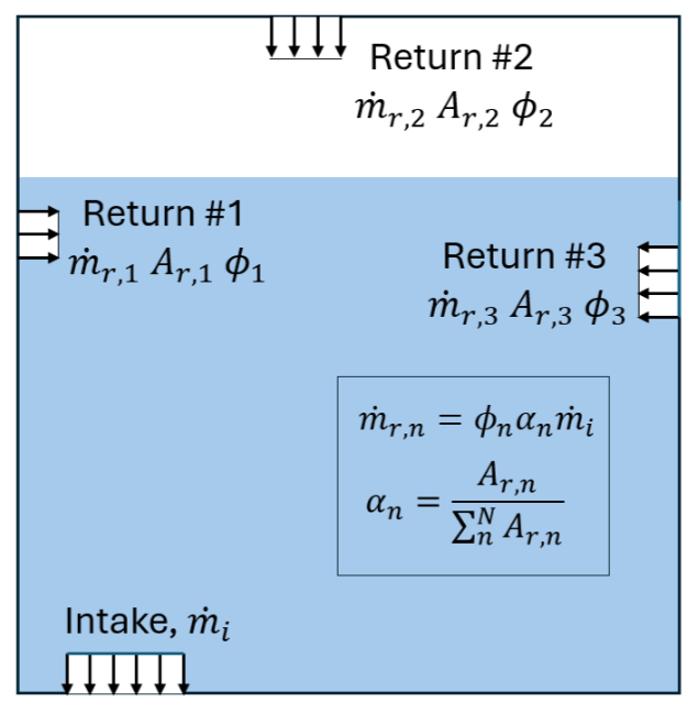
Notional recirculation system with multiple recirculation returns
Download Sample File:
{Inlet/Outlet} Return Value
Examples
Example 1: Continuous Scalar Addition
In this example, the initial (background) scalar concentration in the vessel is zero but the inlet scalar boundary condition has a non-zero specified value scalar concentration. The exit boundary condition is set to a zero gradient condition. The ongoing effects of species mixing cause the concentration to vary across the vessel over space and time. Eventually, the mean concentration across the fluid converges to a steady state value. At this steady state, the scalar flow rate into the system is equal to the scalar flow rate out of the system. In the limit of a perfectly mixed system, the concentration at the zero-gradient outlet condition would be equal to the mean concentration in the vessel.
Download Sample File: Continuous Scalar Addition
Example 2: Continuous Scalar Washout
In this example, the initial (background) scalar concentration in the vessel is non-zero but the inlet scalar boundary condition has a specified value scalar concentration of zero. The exit boundary condition is set to a zero gradient condition. This setup represents a washout process. The ongoing addition of the (scalar-free) inlet fluid causes the mean scalar concentration within the vessel to decrease in time. The concentration at the zero gradient outlet boundary condition varies in space and time due to the ongoing effects of mixing and dilution. Eventually, the washout is complete and the mean scalar concentration converges to zero.
Download Sample File: Continuous Scalar Washout
Example 3: Scalar Recirculation
In this example, a bolus of scalar is added to a vessel with an initial (background) scalar concentration equal to zero. The exit boundary condition is set to a zero gradient while the inlet is configured as a full scalar recirculation return. The simulation is configured with a recirculation delay of four seconds. Physically speaking, this delay represents the time required for the scalar field to transit through recirculation line. The ongoing effects of recirculation cause the scalar field to blend over time. The concentration at the zero-gradient outlet boundary condition varies in space and time due to the ongoing effects of this mixing process. In the limit of a perfectly mixed system, the concentration at the zero-gradient outlet condition would be equal to mean concentration in the vessel.
Download Sample File: Scalar Recirculation