Theory and Implementation

Introduction

The M-Star Solver is a lattice-Boltzmann-based computational fluid dynamics tool used to solve the time-dependent Navier-Stokes equations. Unlike conventional CFD tools, which describe the variation and transport of macroscopic flow variables (e.g. velocity and pressure) across a flow domain, lattice-Boltzmann is a mesoscopic modeling tool that describes the space-time dynamics of a probability distribution function across phase-space. This mesoscopic approach, which is inherently time-dynamic, enables superior turbulence modeling capabilities, faster run times, and scales more favorably with increasing system complexity. The purpose of this section is to summarize the physics governing fluid transport in the solver.

The Boltzmann Equation

M-Star CFD solves the Boltzmann transport equation, which describes the time-evolution of the molecular probability density function \(f\) in phase space [1,2]:

\[\label{1} \frac{\partial f}{\partial t}+\zeta \nabla_x f + K \nabla_\zeta f = Q(f,f)\]

where \(f(x,t)\) is the probability function, \(\zeta\) are the microscopic velocities, \(K\) is any external body force, and \(Q(f,f)\) is a collision operator.

The probability density here corresponds to an ensemble of molecules. As such, \(f dx d\zeta\) is the number of molecules with molecular velocity \(\zeta\) at location \(x\) at time \(t\). Macroscopic variables can be recovered from moments of the distribution function, such as density

\[\label{2} \rho\left({x},t\right)=\int f \left({x},\zeta,t \right)d\zeta\]

and momentum

\[\label{3} \rho {u}\left({x},t\right)=\int \zeta f \left({x},\zeta,t \right)d\zeta\]

The collision operator \(Q(f,f)\) is very complex for an n-body molecular system. But, as argued by Bhatnagar, Gross, Krook (1954), the net effect of this many-body collision should be to drive the local distribution function towards an equilibrium distribution.

\[\label{4} \frac{\partial f}{\partial t}+\zeta \nabla_x f = -\frac{1}{\tau}\left(f-f^0 \right)\]

where \(f^0\) is the so-callled equilibrium probability function and \(\tau\) is the relaxation time.

The relaxation time describes how quickly the distribution relaxes to its equilibrium state over time. This relaxation time, along with the simulation time-step and resolution, will be linked to the local fluid viscosity. Note that, although the external the body force has disappeared, it will return to inform the equilibrium distribution.

Discretization

In Sec\(.\) [1], we assumed that the distribution functions are continuous across \(\zeta\) and \(x\). That is, molecules can assume any position and any velocity vector (quantum limits notwithstanding). In order to make the algorithm tractable, we choose to discretize the molecular velocities into a finite number of velocity vectors. That is, instead of being able to assume arbitrary velocity vectors, individual molecules can only realize velocities defined from a pre-defined set [1-3]:

\[\begin{split}\label{5} \frac{\partial f_i}{\partial t}+\zeta_i \nabla_x f_i = -\frac{1}{\tau}\left(f_i-f_i^0 \right),\\\end{split}\]

where the \(i\) subscript implies a specific velocity vector. Although individual velocities are discretized, the ensemble average velocity can assume any value.

The choice of discrete vectors is not arbitrary. Only specific groups of velocity vectors will maintain isotropic flow conditions and, in the macroscopic limit, recover the Navier-Stokes equations. One suitable set of velocity vectors, called the D3Q19 basis. Other stable basis sets, including D3Q15 and D3Q27 are also available. We find that the D3Q19 lattice provides the best balance between stability and speed.

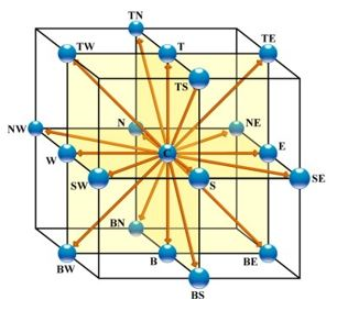
Figure 1: The D3Q19 basis. Individual molecules can only assume any of these velocities. When centered about a given lattice point, each velocity vector points to a nearest neighbor.

Using a forward Euler expansion along each of these discrete velocity vectors, we can re-cast Eqn\(.\) [5] into:

\[\label{6} \frac{f_i\left(x, t+\Delta t \right)-f_i\left(x, t\right)}{\Delta t}+\zeta \left(\frac{f_i\left(x+c_i\Delta t, t+\Delta t \right)-f_i\left(x, t +\Delta t \right)}{\Delta x}\right)=-\frac{1}{\tau}\left(f_i-f_i^0 \right)\]

where \(\Delta x\) is a discrete lattice spacing, \(\Delta t\) is a time-step.

Non-dimensionalizing the molecular velocity by these discretization parameters then gives:

\[\label{7} f_i\left(x+c_i\Delta t, t+\Delta t \right)- f_i\left(x, t \right)=\frac{1}{\tau}\left(f_i-f_i^0 \right),\]

where \(\tau\) has become non-dimensional and \(c_i\) is the non-dimensional lattice velocity, defined by:

\[\label{8} c_i \equiv \zeta_i \frac{\Delta x}{\Delta t}.\]

As presented in Eqns\(.\) [2] and [3], we can recover macroscopic variables from:

\[\label{9} \rho\left({x},t\right)=\sum_{i=0}^N f_i\]

and momentum

\[\label{10} \rho {u}\left({x},t\right)=\sum_{i=0}^N c_i f_i\]

Equilibrium Distribution Function

Since fluid molecules follow Maxwellian statistics, the equilibrium distribution function follows from the Maxwell distribution:

\[f^M=\rho \left( \frac{m^2}{2 \pi R T}\right)^{3/2} e^{\frac{-\left({\zeta}-{u}\right)^2 m^2}{2RT}}, \label{11}\]

where \(m\) is the molecular mass, \(R\) is the gas constant, \(T\) is the temperature, \({\zeta}\) is the molecular velocity, and \({u}\) is the macroscopic flow velocity. In the limit of low Mach numbers, we can use a third-order Taylor expansion to recast Eqn\(.\) [11] as:

\[f^0=\frac{\rho}{\left( 2 \pi R T\right)^{(3/2)}}e^{\frac{-{\zeta}^2}{2RT}}\left(1+\frac{{\zeta} \cdot {u}}{RT} +\frac{\left({\zeta} \cdot {u}\right)^2}{2\left(RT\right)^2}-\frac{{u}^2}{2RT}\right), \label{12}\]

which, for systems with discrete velocity vectors becomes:

\[f_i^0=t_i\rho \left(1+\frac{3}{c^2}\left({c}_i\cdot {u}\right)+\frac{9}{2 c^4} \left({c}_i\cdot {u}\right)^2-\frac{3 {u}^2}{2c^2} \right), \label{13}\]

where \(i\) is an index over the discrete velocity space, \(t_i\) is a weighting index for each vector, and \(c_i\) represent the allowable velocity vectors.

Following Fig\(.\) 1, the weights for the D3Q19 model are:

\[\begin{split} \label{14} t_i= \begin{cases} 1/3,& \text{if } i = C\\ 1/18,& \text{if } i = N,S,E,W,T,B\\ 1/36 & \text{otherwise} \end{cases}\end{split}\]

The Algorithm

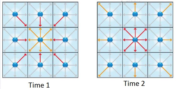
Figure 2: Streaming probability between nearest neighbors.

Streaming

Time integration involves two components: (i) streaming and (ii) collision. The streaming process is illustrated in Fig\(.\) 2: the orange distribution at the center lattice point moves to the nearest neighbor lattice sites, while red distributions come from the nearest neighbor lattice to occupy the velocity vectors at the center lattice. By design, the allowable velocity vectors point to directly nearest neighbors. The processes is representative of molecules streaming between neighboring domains. Because this process occurs on a lattice with characteristic spacing \(\Delta x\) over a characteristic time step \(\Delta t\), it defines a lattice velocity, \(u_{LB}\):

\[\label{15} u_{LB}=\frac{\Delta x}{\Delta t}.\]

Mathematically, \(u_{LB}\) is the speed at which information (probability) moves through the domain. Physically, \(u_{LB}\) can be interpreted as the speed of sound and will inform the compressibility of the fluid.

Collisions

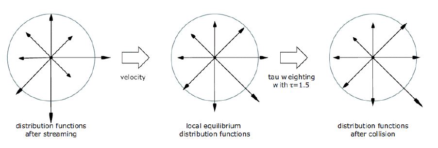
Figure 3: Collision and relaxing towards equilibrium

Following the streaming exchange between nearest neighbor lattice points, the newly arrived distributions at each lattice site undergo a collision process. The collision process, as illustrated in Fig\(.\) 3, drives the molecular distribution function towards the equilibrium distribution function at rate defined by \(\tau\) (see Eqn\(.\) [5]). The equilibrium distribution function is unique to each lattice site and is informed by the local (and instantaneous) macroscopic density and velocity (see Eqn\(.\) [13]). Although the relaxation process modifies the distribution of molecules across the velocity basis vectors, it does not change the macroscopic density and velocity.

Mathematically, the time scale associated with the collision process is assumed to be short compared to the time scale associated with streaming. Physically, this implies that the fluid is operating in low Knudsen number regime (a continuum).

Recall that a low Mach number assumption was evoked when expanding the Maxwell distribution to arrive Eqn\(.\) [12]. Thus, the algorithm presented here is strictly valid in low Knudesen number, low Mach number regimes. Alternative Boltzmann-based approaches for modeling fluids at higher Knudsen numbers and Mach numbers are available in the literature.

Process Flow

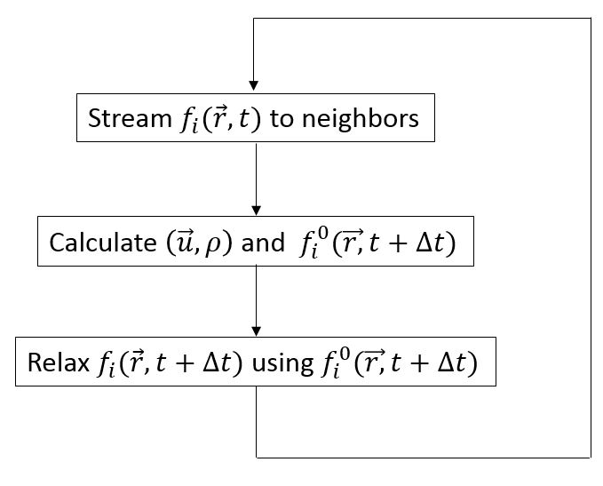
Figure 4: Algorithm work-flow

The origins of the name “Lattice-Boltzmann” should by now be apparent: the Boltzmann transport equation is solved along an array of lattice points stretching across the domain.

Lattice-Boltzmann and Navier-Stokes

Chapman-Enskog Expansion

The link between the (mesoscopic) boltzmann transport equation and the (macroscopic) Navier Stokes equations begins with a Chapman-Enskog (CE) expansion. The CE expansion recognizes that different transport process occur over different length and time-scales. For example, transport due to fluid advection typically occurs at faster time scale than transport due to fluid diffusion. Following this logic, the time derivative associated with transport can be expanded to give [1-3]:

\[\label{16} \partial_t = \epsilon\partial_{t_o}+\epsilon^2\partial_{t_1}+\epsilon^3 \partial_{t_2},\]

and the lattice weights can be expanded to give:

\[\label{17} f_i=f_i^{(0)}+\epsilon f_i^{(1)}+\epsilon^2 f_i^{(2)}+\epsilon^3 f_i^{(3)},\]

where \(\epsilon \ll 1\) is identified as the Knudsen number. Also, since each transport processes occur over the same spatial length scale, the gradient operator becomes:

\[\label{18} \nabla = \epsilon \nabla_1\]

With these expansions in mind, Eqn\(.\) [7] can be recast as a Taylor series:

\[\label{19} \displaystyle \sum_{n=1}^\infty \frac{1}{n!}\left(\partial_t+\textbf{c}_i\cdot \nabla \right)^n f_i=-\frac{1}{\tau}\left(f_i-f_i^0 \right).\]

Injecting the expansions presented in Eqns\(.\) ([16]) to ([18]) into this Taylor series and grouping by powers of \(\epsilon\) gives:

\[\label{20} \left( \partial t_{0}+\mathbf{c}_i \cdot \nabla \right) f_i^{(0)}=-\frac{1}{\tau}f_i^{(1)}\]

and

\[\label{21} \partial_{t_i} f_i^{(0)}+\left( \partial t_{0}+\mathbf{c}_i \cdot \nabla \right) f_i^{(1)}+\frac{1}{2}\left( \partial t_{0}+\mathbf{c}_i \cdot \nabla \right)^2 f_i^{(0)}=-\frac{1}{\tau}f_i^{(2)},\]

for orders \(\epsilon\) and \(\epsilon^2\), respectively.

Recovering Navier-Stokes

The expansions presented in Eqn\(.\) [20] and Eqn\(.\) [21] can be summed over \(i\) to give:

\[\label{22} \partial_{t_0} \rho +\nabla \cdot \left(\rho {u} \right)=0,\]

and

\[\label{23} \partial_{t_0} \left(\rho {u} \right) + \nabla \cdot \Pi^{0}=0.\]

These same expressions (presented in Eqn\(.\) [20] and Eqn\(.\) [21]) can also be multiplied by \(\mathbf{c}\), then summed over \(i\) to give:

\[\label{24} \partial_{t_1} \rho =0,\]

and

\[\label{25} \partial_{t_1} \left(\rho {u} \right) + \left(1-\frac{1}{2 \tau} \right)\nabla \cdot \Pi^{(1)}=0.\]

In Eqns\(.\) [23] and [25], \(\Pi\) is a tensor with the components:

\[\label{26} \Pi_{\alpha \beta}=\displaystyle \sum_i c_{i \alpha} c_{i \beta} f_i,\]

The two timescales can now be superimposed. Begin by combining Eqn\(.\) [22] with Eqn\(.\) [23] to recover the continuity equation:

\[\label{27} \partial_t \rho + \nabla \cdot \left(\rho \vec{u} \right)=0.\]

Then, combine Eqn\(.\) [22] with Eqn\(.\) [23] to recover the momentum equation:

\[\label{28} \partial_t \left(\rho \vec{u} \right) + \nabla \cdot \left(\rho \vec{u} \vec{u} \right)=- \nabla p + 2\nu \nabla \cdot \left(\rho \mathbf{S} \right),\]

where \(\nu=c_s^2\left(\tau - 1/2\right)\) is the lattice kinematic viscosity of the fluid, \(P=c_s^2 \rho\) is the equation of state, and the strain rate tensor is given by:

\[\label{29} S_{\alpha \beta}=\frac{1}{2}\left(\partial_\alpha u_\beta+ \partial_\beta u_\alpha \right).\]

Note that the lattice kinematic viscosity is defined as:

\[\label{30} \nu=\nu_{\textrm{SI}}\frac{\Delta t}{\Delta x^2},\]

where \(\Delta t\) and \(\Delta x\) are the physical lattice spacing and timestep, and \(\nu_{\textrm{SI}}\) is the molecular fluid viscosity.

Strain and Shear Rates

For incompressible (low Mach number) fluids that are continuous (low Knudsen number), Eqn\(.\) [28] can be recast as:

\[\label{31} \rho \partial_t u_\alpha = -\partial_\beta M_{\alpha \beta},\]

where \(M\) is a momentum flux tensor defined by

\[\label{32} M_{\alpha \beta}=p \delta_{\alpha \beta}+\rho u_\alpha u_\beta-\sigma_{\alpha \beta},\]

where \(\delta_{\alpha \beta}\) is the Kronecker delta. The first and second terms in Eqn\(.\) [32] describe the isotropic pressure and momentum transfer due to mass transport. The third term is the shear stress tensor, which takes the form:

\[\label{33} \sigma_{\alpha \beta}=\rho \nu \left( \partial_\alpha u_\beta+\partial_\beta u_\alpha \right).\]

Recognize that, for Newtonian fluids, the strain rate tensor \(S\) in Eqn\(.\) [33] is related to the shear rate tensor presented in Eqn\(.\) [28] through:

\[\label{34} \mathbf{\sigma}=2\rho \nu \mathbf{S}\]

The momentum flux tensor \(\mathbf{M}\) can be recovered from the second moments of \(f_i\). The equilibrium populations recover the first and second terms in Eqn\(.\) [27] (the isotropic pressure and momentum transfer due to mass transport):

\[\label{35} \Pi_{\alpha \beta}^{(0)}=\displaystyle \sum_i c_{i\alpha}c_{i\beta}f_i^{(0)}=c_s^2\rho \delta_{\alpha \beta}+\rho u_\alpha u_\beta.\]

The shear stress is then given by:

\[\label{36} \Pi_{\alpha \beta}^{(1)}=\displaystyle \sum_i c_{i\alpha}c_{i\beta}f_i^{(1)}=-\frac{\tau}{3 \nu}\sigma_{\alpha \beta}.\]

Recognizing that the tracelessness nature of the tensor can be enforced by writing:

\[\label{37} \sigma_{\alpha \beta}=\displaystyle -\left(1-\frac{1}{2 \tau} \right) \sum_i \left( c_{i\alpha}c_{i\beta} - \frac{\delta_{\alpha \beta}}{D} \mathbf{c}_i \cdot \mathbf{c}_i \right)f_i^{\textrm{neq}},\]

where \(f_i^{\textrm{neq}}\) represents the non-equilibrium components of the distribution function. Thus, the shear stress can be assessed locally and independently of the velocity field.

Turbulence Modeling

In principle, the linearized Boltzmann transport equation presented in Eqn\(.\) [7] provides an approach for solving the Navier-Stokes equations is the absence any turbulence model. In practice, however, the stability requirements contained in the recovery of Eqn\(.\) [28] include the provision \(\tau>0.5\). More specifically, since

\[\label{38} \tau=\frac{\nu}{c_s^2}+\frac{1}{2}=\frac{\nu_{SI}}{c_s^2}\left(\frac{\Delta t}{\Delta x^2}\right)+\frac{1}{2},\]

the value of

\[\label{39} \frac{\nu_{SI}}{c_s^2}\left(\frac{\Delta t}{\Delta x^2}\right),\]

must exceed machine precision by multiple orders-of-magnitude. Thus, for a given lattice spacing and timestep, decreasing the molecular viscosity tends to decrease the ratio defined by Eqn\(.\) [39] towards a numerically unstable regime. Although stability can be maintained by either deceasing the timestep and/or resolution, the resolutions required to keep low viscosity (high Reynolds number) systems stable can quickly become impractical to run.

A more practical approach to running lower viscosity (higher Reynolds number) simulations is to activate an LES turbulence filter. An LES turbulence filter operates by superimposing a so-called eddy viscosity, \(\nu_e\), onto the fluid viscosity when solving Eqn\(.\) [28]. The eddy viscosity is informed by the local (and instantaneous) strain field [1-3]`:

\[\label{40} \nu_e=c^2 \Delta x^2 \sqrt{\mathbf{S}:\mathbf{S}},\]

where \(c\) is the dimensionless Smagorinsy coefficient (typically set to a value between 0.1 and 0.2) and \(S\) is defined in Eqn\(.\) [29]. The effects of the LES filter on the local flow field can be characterized by examining the ratio of the fluid viscosity to the total viscosity:

\[\label{41} R_s\equiv\frac{ \nu}{\nu +\nu_e }\]

Likewise, the fraction of energy dissipation resolved by the simulation, \(R\), is be charactered by the ratio:

\[\label{42} R_e\equiv\frac{ 2 \nu \left(\mathbf{S}:\mathbf{S}\right) }{2 \nu \left(\mathbf{S}:\mathbf{S}\right)+2 \nu_e \left(\mathbf{S}:\mathbf{S}\right)} = \frac{\nu}{\nu+\nu_e},\]

Fluid-Structure Interactions

Moving Surfaces

Interactions between the fluid lattice and moving objects are treated using the immersed boundary method. [5] Within this approach, the moving object is modeled as a cloud of Lagrangian points that occupy arbitrary positions within the lattice domain, as illustrated in Fig\(.\) 5. Unlike the flow field, which is only evaluated at fixed and uniform lattice points, the coordinates of each Lagrangian point are continuous and can move over time. The coupling between this Lagrangian point cloud and the fluid lattice involves the application of Newtons second law and an enforcement of the no-slip boundary condition. More specifically, for the lattice points surrounding each immersed boundary point, the algorithm calculates the body force that must be applied to each lattice point to ensure that the fluid velocity (at the interpolated position of the immersed boundary point) is equal to the velocity of the immersed boundary point.

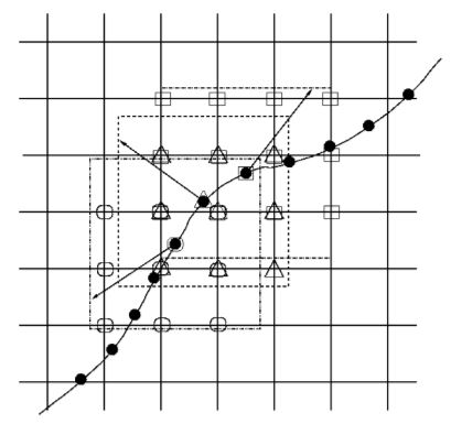
Figure 5: An immersed surface defined by Lagrangian points, along with the corresponding lattice neighborhood. Adapted from [5]

This algorithm is discussed in detail with an appeal to the following definitions. Let \(\mathbf{u^p}\) describe the macroscopic momentum field calculated from Eqn\(.\) [3], prior to any interactions with the moving wall. Let \(\mathbf{X}_k(t)\) describe the position of immersed boundary point \(k\) at time \(t\). Let \(\mathcal{I}[\mathbf{u^p}]\mathbf{X}_k(t)\) define the (interpolated) velocity of the fluid field at the positions \(\mathbf{X_k}\). Using these definitions, we can define the force vector:

\[\label{43} \mathbf{F_{ib}}\left[\mathbf{X}_k(t)\right]=\frac{\mathbf{U^d}\left[\mathbf{X}_k(t)\right]-\mathcal{I}[\mathbf{u^p}]\mathbf{X}_k(t)}{\Delta t},\]

where \(\mathbf{U^d}\left[\mathbf{X}_k(t)\right]\) is the velocity of the immersed boundary point \(k\) at time \(t\) (as imposed by a a user-defined equation of motion), and \(\mathbf{F_{ib}}\left[\mathbf{X}_k(t)\right]\) is the body force that is applied to the fluid at time \(t\) (at each interpolated position \(\mathbf{X}_k\)). Note that Eqn\(.\) [43] is Newton’s second law, and quantifies the force that must be applied to the fluid to ensure that the difference between the fluid velocity vector and the solid object velocity vector is zero.

An interpolation algorithm is need to calculate \(\mathcal{I}[\mathbf{u^p}]\mathbf{X}_k(t)\), and then to project \(\mathbf{F_{ib}}\left[\mathbf{X}_k(t)\right]\) back onto the discrete points of the lattice. We define this interpolation algorithm, \(D\), as necessary to satisfy:

\[\label{44} \mathbf{f}_j(t)=\mathbf{F_{ib}}\left[\mathbf{X}_k(t)\right]D\left[\mathbf{x}_j-\mathbf{X}_k\right],\]

where \(\mathbf{f}_j(t)\) is the body force applied to lattice point \(j\) at time \(t\), \(\mathbf{x}_j\) is the location of the lattice point. Restrictions exist on the functional form of the interpolation algorithm. [5] One acceptable algorithm, which is implemented here, is given by:

\[\begin{split}\label{45} D(r)= \begin{cases} \frac{1}{3}\left(1+\sqrt{-3r^2+1} \right),& \text{if } |r| \leq 0.5\\ \frac{1}{6}\left(5-3 |r|-\sqrt{-3\left(1-|r| \right)^2+1} \right),& \text{if } 0.5 < |r| \leq 1.5\\ 0, & \text{otherwise,} \end{cases}\end{split}\]

where \(r\) is the signed difference between the lattice point and the immersed boundary point. This same interpolation algorithm is used to evaluate the velocity at the location of the immersed boundary point, as applied in Eqn\(.\) [43].

Once \(\mathbf{f}_i(t)\) is calculated for each lattice point, it is projected on the discrete velocity vectors \(i\) at each lattice site via:

\[\label{46} F_{j,i}(t)=\left(1-\frac{1}{2\tau} \right) t_i \left[\left(\frac{{c}_i-{u}}{c^2}\right)+\left(\frac{{c}_i \cdot {u}}{c^4}\right){c}_i \right] \cdot \mathbf{f}_j(t),\]

where \(F_{j,i}(t)\) is the body force applied to lattice point \(j\) along the discrete velocity vector \(i\) at time \(t\). Recall the \(t_i\) is the weighting factor introduced in Eqn\(.\) [13].

This body force is added to the right-hand side of Eqn\(.\) [7] to give:

\[\label{47} f_i\left(x+c_i\Delta t, t+\Delta t \right)- f_i\left(x, t \right)=\frac{1}{\tau}\left(f_i-f_i^0 \right)+F_i(t),\]

as the governing LBM equation at each lattice point \(j\) for systems with moving boundaries.

Static Surfaces

Figure 6: Bounce-back boundary conditions work flow.

Non-moving, static surfaces are modeled using the mid-way bounce-back approach.:raw-latex: [6] Under this approach, any portion of the probability density function that interacts with a bounce-back (wall) node is reflected back into the fluid along its incoming direction. As illustrated in Fig\(.\) 6, the actual position of the boundary is mid-way between the nearest “wet” node that a set of ghost nodes positioned behind the boundary. Probability that crosses the wall moves into the ghost nodes, relaxes, and then is reflected back into the fluid. Although this approach requires the introduction of extra lattice (in the form of ghost lattice points), it is second-order of accurate.

Scalar Transport

The Convection-Diffusion Equation

Species transport at each lattice point \(i\) is modeled via the convection-diffusion equation:

\[\label{48} \frac{\partial c}{\partial t}= \nabla \cdot \left( D \nabla c \right)-\nabla \cdot \left({v} c \right)+R\]

where \(c\) is the concentration of the scalar field, \(D\) is the diffusion coefficient, \({v}\) is the macroscopic velocity field, and \(R\) is a source/sink term.

Equation [48] is solved using a flux conserving scheme. Within this scheme, each lattice point defines the center of a cubic cell that exchanges species with neighboring cells through its six cell walls. If the total volume, \(V\), of each cell is defined as:

\[\label{49} V=\Delta x \Delta x \Delta x\]

then the amount of scalar field defined each cell is defined as:

\[\label{50} Q_i=c_i V.\]

For each cubic cell, the change in \(Q_i\) over time is governed by the flux exchange between neighbor cells:

\[\label{51} \frac{d Q_i}{dt}=\left(f_{i,x-1/2}-f_{i,x+1/2}+f_{i,y-1/2}-f_{i,y+1/2}+f_{i,z-1/2}-f_{i,z+1/2}\right) \cdot S,\]

where the \({i,x-1/2}\) subscript indicates the position of the interface relative to the cell center, \(f\) is the flux, and \(S\left(=\Delta x \Delta x \right)\) is the surface area of the cell.

Recognizing that this update is done at the half-time, and linearizing the time-derivative gives:

\[\label{52} c_i^{t+1}=c_i^{t}+\frac{\Delta t}{\Delta x}\left(f_{i,x-1/2}^{t+1/2}-f_{i,x+1/2}^{t+1/2}+f_{i,y-1/2}^{t+1/2}-f_{i,y+1/2}^{t+1/2}+f_{i,z-1/2}^{t+1/2}-f_{i,z+1/2}^{t+1/2}\right) \cdot S,\]

Per the Lax Equivalence Theorem, the functional form of \(f\) in Eqn\(.\) [51] is not arbitrary; the algorithm used to define \(f\) must be both stable and consistent. [8] One option for ensuring stability, called the Lax-Wendroff algorithm, is to add precisely enough artificial viscosity to keep the algorithm stable. A second option for ensuring stability is to define a van Leer flux limiter, which performs second-order advection in regions where the flow field is smooth, and donor-cell advection near gradients. For highly turbulent systems dominated by scalar advection, the behavior of both algorithms is similar. For laminar or transitional systems, where diffusion must be controlled, the van Leer flux limiter should be used.

Particle Transport

Particles are modeled as discrete point masses with trajectories governed by Newton’s Second Law:

\[\label{53} m_i \frac{d{v}}{dt}=\displaystyle \sum {F}_i={F}_g+{F}_b+{F}_d+{F}_p,\]

where \(m_i\) is the mass of particle, \({v}\) is the velocity, \({F}_g\) is the gravity force, \({F}_b\) is the buoyancy force, \({F}_d\) is the drag force with the fluid, and \({F}_p\) is the inter-particle collision force. The local drag force is valuated using literature sphere drag data [8]. Although inter-particle collisions are modeled as hard-sphere interactions by default, it is straightforward to extend these interactions to model aggregation and break-up. Note that particle dynamics are not confined to the lattice, and they can occupy arbitrary positions and velocity vectors.

References

[1] S. Succi. The lattice Boltzmann equation for fluid dynamics and beyond, Oxford: Oxford University Press, 2001.

[2] C. Shu and Z. Guo. Lattice Boltzmann method and its applications in engineering. New Jersy: World Scientific, 2013.

[3] T. Kruger, H. Kusumaatmaja, A. Kuzmin, O. Shardt, G. Silva, and E. Viggen. The lattice Boltzmann method: principles and practice. Switzerland: Springer, 2017.

[4] Z. Feng and E. Michaelides. J. Comp. Phys., 195(2):602-628, 2005

[5] C. Peskin. Acta Math., 11:479-517, 2002

[6] M. Sukop and D. Thorne. Lattice Boltzmann Modeling: an Introduction for Geoscientists and Engineers, Heidelberg: Springer, 2006

[7] R. LeVeque. Finite Volume Methods for Hyperbolic Problems, Cambridge University Press, 2002

[8] A. Morrison. An Introduction to Fluid Mechanics, Cambridge University Press, 2013