Choosing a Simulation Resolution: Agitated Tanks

Objective

In this work, we will use M-Star CFD to predict the effects of resolution on power number across a range or Reynolds numbers for multiple impellers. From this output, we will provide guidance on recommended simulation resolutions.

Input Files

Input file available here

Conceptual Overview

Within the context of the lattice-Boltzmann method, two simulation parameters must be specified: simulation resolution and simulation time step. The simulation resolution, which is discussed here, informs the hydrodynamic length scales that can be captured by the simulation. The simulation time step, as discussed in a separate module, informs the compressibility of the fluid. In principle, increasing the lattice resolution tends to increase the fineness of the fluid structures that can be resolved by the simulation. In practice, however, this increase leads to more computationally demanding models. An engineering balance between resource and simulation fidelity must be considered when building the model.

To understand this balance, here we assess the effects of simulation resolution on power number across a range of Reynolds numbers for three impellers: Rushton, pitch blade turbine, and low-solidity hydrofoil. We compare the predictions to experimental data, then use this resolution study to provide guidance on simulation resolutions.

Note

• The terms simulation resolution and lattice spacing are related. The lattice spacing is a measured quantity that describes the physical distance between two lattice points. The simulation resolution is a dimensionless integer describing the number of lattice points across a relevant system length scale. For a fixed-system length scale, increasing the simulation resolution decreases the lattice spacing.

Recall that the power number, $N_p$, is a non-dimensional parameter defined by:

$$N_p=\frac{\tau \omega }{\rho N^3{D}^5},$$

where $\tau$ is the torque on the impeller, $\omega$ is the angular velocity, $\rho$ is the fluid density, $N$ is the impeller speed, and $D$ is the impeller diameter. Note that $\tau$ and $\omega$ are often measured in N-m and radians/second, while $\rho$, $N$, and $D$ are measured in kg/m³, revolutions per second, and meters. The power number is useful in estimating strain and energy dissipation rates within the vessel. That is, owing to the conservation of energy, the total energy dissipation rate within the fluid must be equal to the power delivered to the fluid by the impeller.

The pumping number, $N_q$, is a non-dimensional parameter defined by:

$$N_q=\frac{Q}{N{D}^3},$$

where $Q$ is the volumetric flow rate of fluid leaving a control volume immediately surrounding the impeller. Note that $Q$ is often measured in m³/s, while $N$ and $D$ are typically measured in revolutions per second and meters. The pumping number is useful in estimating blending and circulation within the vessel. That is, owing to the conservation of mass, the pumping action of the impeller can be related to tank blend time. A notional control volume is illustrated in powerPumpingNumberImage.

Conceptual description of the power number (defined from the torque on the shaft) and pumping number (defined by the control volume flux).

To contextualize this discussion, in powerNumberVersusRe, we present the measured power number for multiple impellers across a range of Reynolds numbers. [Ma] This data was generated using a standard impeller-to-tank diameter ratio of 1:3, with the impeller located one impeller diameter off the tank bottom. The tank was baffled with a fluid height equal to the tank diameter. Each impeller power number follows three general trends:

1. In the laminar regime (Re<10), the power number decreases inversely with Reynolds number.

2. In the transitional regime (10<Re<1000), the power number converges towards a plateau.

3. In the turbulent regime (Re>1000), the power number is largely independent with Reynolds number.

Observe the order-of-magnitude increase in power number with decreasing Reynolds number. Also observe that, across the entire Reynolds number spectrum, hydrofoils have lower power numbers than pitch blade turbines, which in turn have lower power numbers then Rushton impellers.

Power number vs Re

Building the Models

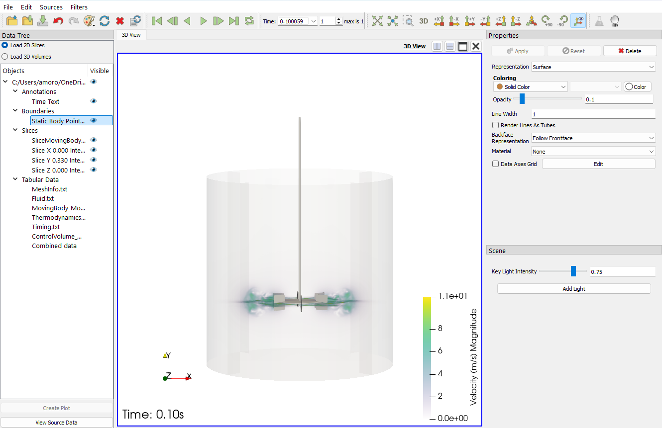
In firstLabel6p, we present an illustration of the simulated system for the Rushton impeller runs. The tank diameter and fluid height were both 1 m, while the impeller diameter was 0.33 m. Between simulations, the impeller speed and fluid viscosity varied from 30 to 300 RPM and 5e-2 to 5e-6 m^2/s to realize target Reynolds numbers. The tank walls had a no-slip boundary condition.

Since the system is baffled with four 0.08-m wide baffles, a surface vortex is not expected to form. As such, the top surface was modeled using a flat free-slip boundary condition. The simulation runtime was set to 20 seconds, a time sufficient to capture steady-state power and flow dynamics. The Courant number was set to 0.05 for all simulations, which ensured that variations in the lattice density remained below 2%. An LES turbulence closure model was applied with the default Smagorinsky coefficient of 0.1. Although each model included this LES filter, its effect in the laminar flow regime is negligible as a DNS solution is recovered. We address this point in detail below.

Power number setup

Analyzing the Output: Power Number

In firstLabel7p, we present power number output from the Rushton impeller simulation across a range of Reynolds numbers. The resolution in each simulation was set to 300 points across the tank diameter, which corresponds to approximately 120 points across the impeller. After a few-second transient stage, during which the fluid is accelerated from rest to a steady-state flow condition, the power number becomes constant. In the laminar flow regime (Re<10), this predicted power number decreases strongly with increasing Reynolds number. In the transitional regime, (10<Re<1000), the predicted power number reaches a minimum. In the turbulent flow regime, (Re>1000), the predicted power number increases slightly with increasing power number. Conceptually speaking, the order-of-magnitude variation in impeller power number with Reynolds number is consistent with experimental data reported in powerNumberVersusRe.

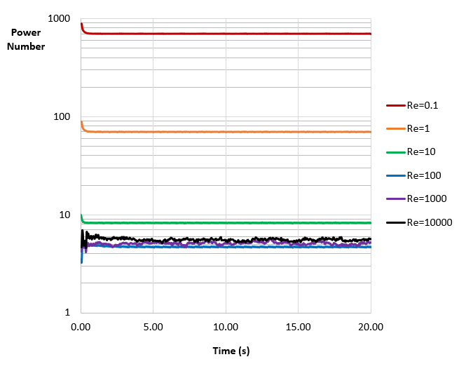
Power number measured experiment

In firstLabel5q we superimpose this steady-state power data on the experimentally measured power number data. To aid in comparison, the power number in both data sets has been normalized by the fully turbulent power number. The fully turbulent power number predicted here for the Rushton impeller was 5.8. This value agrees with the reported values of 5-6 for similar impeller designs, as well as the 5.41 value reported for the experimental set here. [] Good agreement is realized between predictions and measurements across the range of Reynolds numbers considered here.

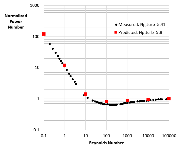
Steady-state power data on the experimentally measured power number data

In firstLabel5pbt and firstLabel5hydrofil, we compare this same data for a pitch blade turbine and a low solidity hydrofoil. Just like the Rushton impeller system, the pitch blade turbine and the hydrofoil show distinct laminar and turbulent flow regimes, with a transitional regime between a Reynolds number of 10 and 1000. The fully turbulent power numbers predicted here for the two impellers were 1.26 and 0.35, respectively. These values agree with the 1.2 and 0.31 values reported in the experimental report. [Ma] Good agreement is also realized across the Reynolds number spectrum.

The generality of this approach is noteworthy: power numbers ranging from 0.35 to 700 across Reynolds numbers ranging from 0.1 to 100,000 were correctly predicted for three topologically unique impellers, with no model tuning or re-parameterization. These results engender confidence in the ability of the solver to predict behavior in more complex systems, involving non-Newtonian rheology and time-varying operating conditions that may transverse multiple Reynolds number regimes.

Pitch blade turbine normalized power number versus Reynolds number

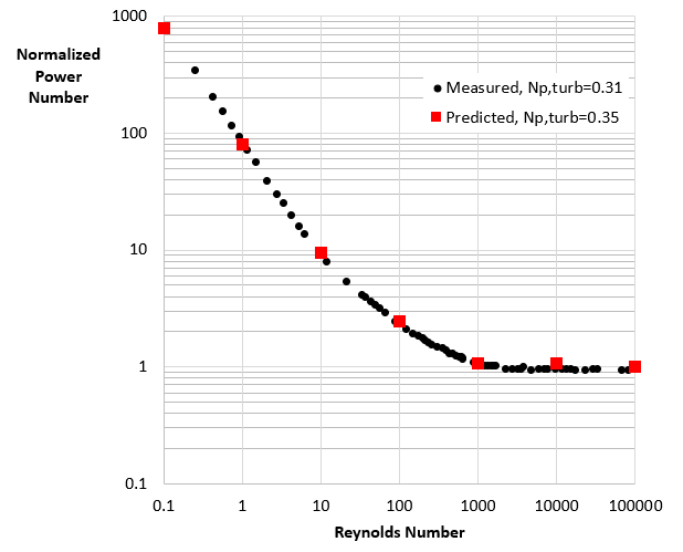
Hydrofoil normalized power number versus Reynolds number

In Figure firstLabel7p, we show the effect of resolution on steady-state power number prediction for each impeller at Reynolds numbers of 1, 100, and 10,000. These three Reynolds numbers were selected to target the laminar, transitional, and turbulent flow regimes. To present a self-similar comparison, we normalize the power number at each resolution by the fully converged value (reported in the legend) for the given operating condition. We recognize that many of these markers overlap, making individual points difficult to discern. The purpose of this plot, however, is to demonstrate a key trend: for all nine systems, the power number converges to within 5% of the fully converged value at a resolution of 250 points per tank diameter. Thus, as a conservative rule, we recommend a lattice resolution of 80–100 lattice points per impeller diameter to correctly predict shaft power and power dissipation in the fluid.

Upon closer examination, we recognize that the Rushton impeller (square markers) requires the fewest lattice points to realize a grid-independent power number. In fact, for each Reynolds number, the Rushton power number converges at a resolution of only 100 lattice points across the tank (50 across the impeller). Similarly, for each Reynolds number, we recognize that the PBT impeller (circle markers) requires only 150 points across the tank (70 across the impeller) to realize a grid-independent power number. Thus, while the 100 lattice-points-per-impeller-diameter is a good conservative rule, it is driven by the low solidity hydrofoil. Coarser (and therefore much faster) simulations are generally sufficient when modeling agitated tanks with flat blades or high solidly impellers.

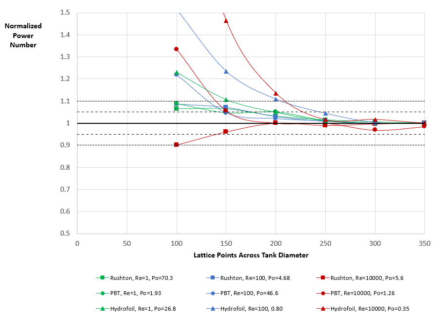
Effect of resolution on predicted power number at multiple Reynolds numbers and impellers

References

[Ma] (1,2)

Ma, Z. 2014. Impeller Power Draw Across The Full Reynolds Number Spectrum. M.S. Thesis. University of Dayton, Department of Chemical and Materials Engineering.

[ChemEng2017]

https://www.philamixers.com/content/uploads/2017/08/Chemical-Engineering-Aug-2017.pdf