Moving Parametric Geometry¶

Moving parametric geometry objects define motion expressions supported by particle, scalar field, and global variable parent objects. For particle and scalar field parents, these objects can define a moving addition. For global variables, these objects can model a moving analysis region. This functionality is illustrated in the examples below.

Property Grid¶

These are the parameters that define the moving child geometry. The categories, settings, and/or selections available within the property grid depend on the child geometry type, as listed in the catalog.

`General`¶

Initial Location: m | The initial position of the center of the boundary condition surface in model units. Displacement UDFs are defined relative to this initial position.

`Motion`¶

Displacement X UDF

m | This UDF defines the X displacement of the moving geometry relative to the initial position. The initial value of the UDF should be zero. This is a System UDF.

Displacement Y UDF

m | This UDF defines the Y displacement of the moving geometry relative to the initial position. The initial value of the UDF should be zero. This is a System UDF.

Displacement Z UDF

m | This UDF defines the Z displacement of the moving geometry relative to the initial position. The initial value of the UDF should be zero. This is a System UDF.

In this example, we model the hand casting of particles above the free surface of an agitated vessel. The position of the moving injection cuboid is described using a sinusoidal trajectory. This functionality can also be applied to bubbles (for modeling moving spargers) as well as DEM particles (for modeling moving particle sources).

Download Sample File: Casting Particles

In this next example involving scalar fields, we model photodegradation via a moving light source. Physically speaking a light beam is moving across a tank causing local species depletion.

Download Sample File: Degradation

For global variables, the moving geometry represents a moving evaluation region. The reductions can be applied to both moving child geometry and static child geometry. In the example below, we use a moving geometry that rotates with the impeller to sample the energy dissipation rate in the trailing vortex behind an impeller blade.

Download Sample File: Moving Evaluation Region

`Geometry`¶

Lx, Diameter, etc.: These are the parameters that define the cuboid, cylinder, or sphere. The exposed parameters will depend on the geometry type, as listed below.

`Display Attributes`¶

Visible

This controls whether the object is displayed in the 3D viewing panel.

Hidden

The object is not displayed in the 3D view.

Shown

The object is displayed in the 3D view.

Mode

This controls how the object is rendered.

Wire

This renders the object as a wireframe.

Color: This sets the color of the wireframe.
Width: This adjusts the line width used to render the wireframe.

Shaded

This renders the object as a shaded surface.

Material: This sets the surface material. Available options are Aluminum, Steel, Chrome, Plastic, and Glass.
Color: This sets the surface color.
Opacity: When glass is selected, this sets surface opacity.

Catalog¶

The catalog below lists the exposed parameters for each geometry type.

Cuboid¶

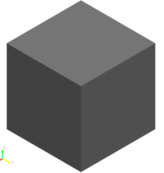
Lx: Length in X direction
Ly: Length in Y direction
Lz: Length in Z direction

Cylinder¶

Diameter: Cylinder diameter
Length: Cylinder Length

Sphere¶

Diameter: Sphere diameter

See Context Specific Toolbar for Child Geometry.