Planes/Probes

The Planes/Probes control panel specifies which field quantities are calculated and exported along Output Planes and Output Surfaces. The panel also controls the corresponding write interval, as well as any conditional output logic. These are used to represent both fluid field data and particle field data.

Plane and surface outputs write spatially resolved field data evaluated on two-dimensional manifolds defined within the lattice. These outputs retain geometric shape, topology, and coordinate information rather than reporting single-valued reduced outputs. Output planes are presented as planar rectangular cross-sections spanning the full three-dimensional lattice, while output surfaces are presented as user-defined two-dimensional manifolds which sample localized regions of the domain.

Plane data are written to binary .vti files for visualization, animation, and analysis within M-Star Post or any compatible VTI file reader. The name of each output file is linked to the Axis Direction and corresponding Intercept Value used to define the plane. Output surface data are written to binary .vtp files, with filenames linked to the dynamic name of the corresponding surface geometry. Both files types are printed at the output Write Interval.

In addition to controlling plane and surface writing frequency, the Write Interval also defines a rendering output frequency for particles, moving bodies, static bodies, and fluid-interface geometry. This makes the output frame-consistent for visualization and animation. When probes are rendered spatially (e.g., for animation), their visualization output is also synchronized with the Write Interval defined here. The ASCII statistics output for probes and output lines, however, is still written at the statistics output interval.

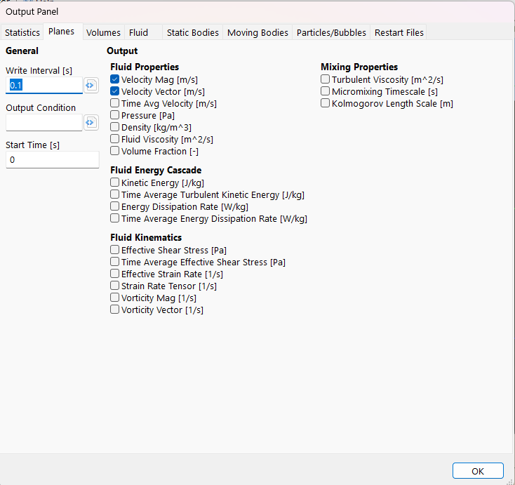
Output Panel

General

Write Interval UDF

s | This UDF defines the interval at which spatial output data are written. This includes plane and surface outputs, as well as rendering output for particles, bodies, free-surface geometry, and spatially rendered probes. The write interval can vary with simulation time, as well as any global variables or global constants. This is a System UDF.

Download Sample File: Write Interval

Tip

Plane output data should be written every 200–1000 time steps to balance the computational overhead of file I/O with the need for sufficient temporal resolution during post-processing.

Warning

Decreasing the Write Interval will increase the amount of disk space required to store the output data.

Note

When producing real-time animations using slice, particle, or free surface data, the animation frame rate should correspond to the reciprocal of the Slice Output Interval. For example, an output rate of 0.05 s would correspond to a frame rate of 20 frames per second, etc.

Output Condition UDF

no units | This UDF defines event conditions that force an immediate write of the spatial output data. This captures output data at specific simulation events and triggers writes in addition to those scheduled by the Write Interval. This is a System UDF.

Download Sample File: Output Condition

Start Time

s | Start time of plane/slice writes.

Output Control

Fluid Properties

These properties define the local state of the flow field and describe how momentum, mass, and phase information evolve throughout the domain.

▢ Velocity Vector

m/s | This defines the three-dimensional fluid velocity vector, \(\vec{V}\), defined as

\[\vec{V}={v_x}\vec{i}+{v_y}\vec{j}+{v_z}\vec{k},\]

where \(v_x\), \(v_y\), and \(v_z\) are the x-, y-, and z-components of the velocity field.

▢ Velocity Magnitude

m/s | This defines the magnitude of the local fluid velocity vector.

▢ Time-Averaged Velocity Vector

m/s | This defines the time-averaged fluid velocity vector, \(\langle \vec{V} \rangle\), calculated as

\[\langle \vec{V} \rangle = \langle v_x \rangle \vec{i} + \langle v_y \rangle \vec{j} + \langle v_z \rangle \vec{k},\]

using the averaging scheme defined in the Time Averaging category within Simulation Parameters.

▢ Pressure

Pa | This defines the local total fluid pressure.

▢ Density

kg/ \(m^3\) | This defines the local fluid density.

▢ Fluid Viscosity

\(m^2\) /s | This defines the local fluid viscosity.

▢ Fluid Volume Fraction

This defines the local fluid volume fraction. If the fluid configuration is set to Immiscible Two Fluid, this output will show the relative volume fractions of both fluid 1 and fluid 2 across the domain. If the fluid configuration is set to Free Surface, this output represents the local fluid volume fraction across the domain and can be used to characterize the topology of the fluid surface or interface. If the fluid configuration is set to Single Phase, this output can be used to assess the effects of the flood fill.

Fluid Energy Cascade

This group of outputs characterizes how kinetic energy is stored, transferred, and dissipated within the flow field across spatial and temporal scales.

▢ Total Kinetic Energy

J/kg | This characterizes the instantaneous kinetic energy of the fluid per unit mass, calculated as

\[k_{total}=\frac{1}{2}|\vec{V}|^2,\]

where \(\vec{V}\) is the local three-dimensional velocity vector.

▢ Time-Averaged Turbulent Kinetic Energy

J/kg | The time-averaged turbulent kinetic energy per unit mass is computed from the fluctuating components of the velocity field

\[k_{\mathrm{tke}} = \frac{1}{2}\left( \langle {v'_x}^2 \rangle + \langle {v'_y}^2 \rangle + \langle {v'_z}^2 \rangle \right),\]

with

\[\left\langle {v'_i}^2 \right\rangle = \frac{1}{\,n - n_s + 1\,} \sum_{m=n_s}^{n} \left( v_i^{(m)} - \left\langle v_i \right\rangle \right)^2, \qquad i \in \{x, y, z\},\]

where the ⟨\(v_i\)⟩ is the time-averaged fluid velocity vector calculated using the averaging scheme defined in Time Averaging within Simulation Parameters. Within the summation, \(n_s\) is the simulation time step corresponding to the Begin Time Average time, \(n\) is the current simulation time step, and \(n−n_s+1\) is the total number of time steps included in the running average.

▢ Energy Dissipation Rate

W/kg | The energy dissipation rate is the rate at which kinetic energy is converted into thermal energy by viscous stresses. The local dissipation rate per unit mass is

\[\varepsilon = 2\nu \, \mathbf{S} : \mathbf{S},\]

where \(\varepsilon\) is the local kinematic viscosity, and \(\mathbf{S}\) is the local strain-rate tensor. The strain-rate tensors used to evaluate the local dissipation rate are evaluated directly from the LBM distribution function. This approach yields a more accurate evaluation of the Frobenius inner product.

▢ Time-Averaged Energy Dissipation Rate

W/kg | This defines the time-averaged energy dissipation rate, calculated from the average scheme defined in Time Averaging within Simulation Parameters.

Fluid Kinematics

This group of outputs describes the local deformation and rotational behavior of the fluid independent of material properties.

▢ Resolved Strain Rate Tensor

1/s | The resolved strain-rate tensor is a second-order tensor computed as

\[S_{ij} = \frac{1}{2}\left( \frac{\partial v_i}{\partial x_j} + \frac{\partial v_j}{\partial x_i} \right).\]

Here, \(v_i\) is the \(i\) -th component of the fluid velocity vector. The strain-rate tensor is evaluated from the velocity field using a finite-difference representation of the velocity gradient.

▢ Resolved Strain Rate

1/s | The resolved fluid strain rate is a scalar quantity computed as

\[\dot{\gamma} = \sqrt{S_{ij} S_{ij}},\]

where \(S_{ij}\) is the resolved strain-rate tensor. This corresponds to the magnitude of the strain-rate tensor based on the Frobenius norm.

▢ Resolved Shear Stress

Pa | The resolved fluid shear stress is a scalar quantity computed as

\[\tau_{\mathrm{mag}} = \sqrt{2\, \tau_{ij}\tau_{ij}},\]

with

\[\tau_{ij} = 2 \rho \nu \, S_{ij},\]

where \(S_{ij}\) is the resolved strain-rate tensor. Here, \(\rho\) and \(\nu\) are the local fluid density.

▢ Time-Averaged Resolved Shear Stress

Pa | The time-averaged resolved shear stress is computed by applying the time-averaging scheme defined in Time Averaging within Simulation Parameters to the resolved shear stress field.

▢ Vorticity Vector

1/s | The vorticity vector is defined as the curl of the velocity field

\[\boldsymbol{\omega} = \nabla \times \vec{V},\]

where \(\vec{V}\) is the local fluid velocity vector.

▢ Vorticity Magnitude

1/s | This defines the magnitude of the local fluid vorticity vector.

Mixing Properties

This group of outputs characterizes sub-grid-scale transport and small-scale mixing behavior that is not directly resolved by the computational mesh.

▢ Sub-Grid Turbulent Viscosity

\(m^2\) /s | The sub-grid turbulent viscosity represents enhanced momentum transport due to unresolved turbulent motions. It is defined as

\[\nu_t = (C_s \Delta)^2 |S|,\]

where \(|S|\) is the resolved strain rate, \(C_s\) is the Smagorinsky coefficient, and \(\Delta\) is the local grid filter width (lattice spacing).

▢ Micromixing Timescale

s | The micromixing timescale characterizes the time required for scalar fluctuations to be homogenized at the smallest turbulent scales. It is computed as

\[\tau_{\mu} = 17.89\, (\nu \varepsilon)^{1/2},\]

where \(\nu\) is the local kinematic viscosity, and \(\varepsilon\) is the local energy dissipation rate. The 17.89 cofactor is taken from the work of Nouri et al.

▢ Kolmogorov Length Scale

m | The Kolmogorov length scale represents the smallest length scale of turbulence at which viscous dissipation dominates. It is defined as

\[\eta = \left(\nu^{3}\varepsilon\right)^{1/4},\]

where \(\nu\) is the local kinematic viscosity, and \(\varepsilon\) is the local energy dissipation rate.

Thermal Properties

This group of outputs describes the thermal state of the fluid and its spatial and temporal variation within the flow field.

▢ Temperature

K | This describes the local thermodynamic temperature of the fluid, expressed in absolute units.

Custom Variables

This group of outputs includes custom and other derived quantities that are not primary flow variables.

▢ Mean Age

s | The mean age represents the average time elapsed since fluid entered the domain or was initialized at the specified reference condition. The mean age \(A(x,t)\) satisfies an advection–diffusion equation with a unit source term

\[\frac{\partial A}{\partial t} + \vec{V} \cdot \nabla A = \nabla \cdot \left( D \nabla A \right) + 1,\]

where \(A\) is local the mean age, \(\vec{ V}\) is the local fluid velocity vector, and \(D\) is the effective age diffusivity. The source term \(1\) represents the continuous accumulation of time over each time step.

▢ Porosity

The local porosity represents the fraction of a control volume that is available for fluid flow. It is defined as the ratio of fluid-filled volume to total volume.

▢ {Voxel Variable}

This describes the local magnitude of the Voxel Variable. The selection name is the Dynamic Name of the associated voxel variable.

Scalar Fields

This group of outputs includes scalar field concentration as well as the associated molecular diffusion coefficients.

▢ {Scalar Field} Concentration

mol/L, volume fraction, g/L | This describes the local species concentration associated with the scalar field. The selection name is the dynamic name given to the scalar field. The units are defined by the Base Unit of the scalar field.

▢ Diffusion Coefficient

\(m^2\) /s | This describes the local diffusion coefficient associated with the named scalar field.