Bubbles/Particles

The Bubbles/Particles Output Panel specifies which particle-resolved and particle-derived quantities are calculated and exported during a simulation.

Particle outputs include both Lagrangian particle data and Eulerian field quantities constructed from the particle population. Individual particle outputs retain spatial position and particle-specific attributes such as shape, composition, size, velocity, forces, and user-defined particle properties. These datasets can also include local fluid properties sampled at the particle location, including strain rate and local energy dissipation rate (EDR). Eulerian particle fields are constructed by mapping the particle population onto the lattice to produce spatial fields such as particle volume fraction, interfacial area, and kLa-related quantities. These fields are written on slice and volume datasets, enabling direct comparison between particle distributions and continuum fluid fields.

All particle visualization outputs are written to binary VTK formats and are synchronized with the Plane/Probe Write Interval as well as the Volume Write Interval. This makes the output frame-consistent for visualization and animation in both 2D and 3D renderings. Each particle set will have a unique output file with a file name linked to the dynamic name of the particle family.

In parallel with spatial outputs, the particle output system can generate exit age and exit location lists for further analysis of particle residence time behavior and exit distributions.

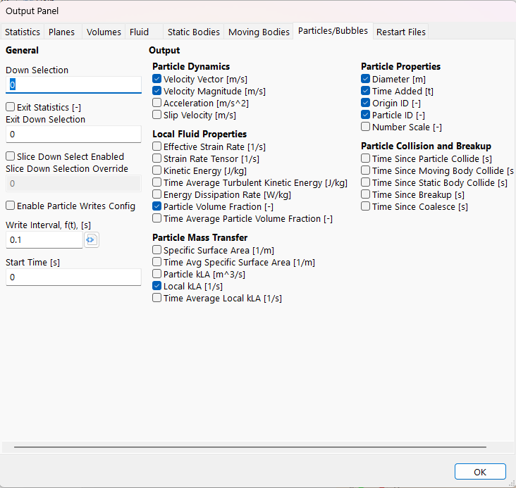
Output Panel

General

Down Selection

This parameter down-selects particle visualization output to every \(N^{th}\) particle to reduce file size and rendering cost. The selected particles are chosen randomly for each output frame and may differ between frames. This option does not affect particle physics or statistical calculations. This output only affects visualization output.

▢ Exit Statistics

Exit Down Selection

This parameter tracks particles that leave the computational domain and records their particle ID, time added, exit time, exit location, and origin ID. When exit down selection is enabled, approximately every \(N^{th}\) exiting particle is recorded in the exit statistics file. Particles are randomly sampled, so the specific set of recorded exits may vary between runs while remaining statistically representative of the full exiting population.

Output Control

Particle Dynamics

These outputs describe the instantaneous motion of each particle, including velocity, acceleration, and slip relative to the surrounding fluid. They are used to quantify particle transport, inertia, and coupling with the fluid flow.

▢ Velocity Vector

m/s | This defines the three-dimensional particle velocity vector, \(\vec{V}_p\), defined as

\[\vec{V}_p = v_{p,x} \hat{i} + v_{p,y} \hat{j} + v_{p,z} \hat{k},\]

where \(v_{p,x}\), \(v_{p,y}\), and \(v_{p,z}\) are the x-, y-, and z-components of the particle velocity vector.

▢ Velocity Magnitude

m/s | This defines the magnitude of the local particle velocity vector.

▢ Acceleration

m/ \(s^2\) | This defines the three-dimensional particle acceleration vector, \(\vec{a}_p\), defined as

\[\vec{a}_p = a_{p,x} \hat{i} + a_{p,y} \hat{j} + a_{p,z} \hat{k},\]

where \(a_{p,x}\), \(a_{p,y}\), and \(a_{p,z}\) are the x-, y-, and z-components of the particle acceleration vector.

▢ Slip Velocity

m/s | This defines the slip velocity

\[\vec{V}_{\text{slip}} = \vec{V}_p - \vec{V}_f,\]

where \(\vec{V}_f\) is the velocity of the fluid surrounding the particle.

Local Fluid Properties

These outputs describe the local motion and deformation of the fluid evaluated at particle locations, based directly on the resolved velocity field, independent of material models such as viscosity or rheology. They quantify local strain, turbulence intensity, and energy dissipation experienced by the particles, which drive mixing, mass transfer, and particle transport.

▢ Resolved Strain Rate Tensor

1/s | The resolved strain-rate tensor is a second-order tensor computed as

\[S_{ij} = \frac{1}{2} \left( \frac{\partial v_i}{\partial x_j} + \frac{\partial v_j}{\partial x_i} \right).\]

Here, \(v_i\) is the \(i\)-th component of the fluid velocity vector. The strain-rate tensor is evaluated from the velocity field using a finite-difference representation of the velocity gradient.

▢ Resolved Strain Rate

1/s | The resolved fluid strain rate is a scalar quantity computed as

\[\dot{\gamma} = \sqrt{2 \, S_{ij} S_{ij}},\]

where \(S_{ij}\) is the resolved strain-rate tensor. This corresponds to the magnitude of the strain-rate tensor based on the Frobenius norm.

▢ Total Kinetic Energy

J/kg | The instantaneous kinetic energy of the fluid per unit mass, calculated as

\[k_{total}=\frac{1}{2}|\vec{V}|^2,\]

where \(\vec{V}\) is the local three-dimensional velocity vector.

▢ Time-Averaged Turbulent Kinetic Energy

J/kg | The time-averaged turbulent kinetic energy per unit mass is computed from the fluctuating components of the velocity field

\[k_{\mathrm{tke}} = \frac{1}{2}\left( \langle {v'_x}^2 \rangle + \langle {v'_y}^2 \rangle + \langle {v'_z}^2 \rangle \right),\]

with

\[\left\langle {v'_i}^2 \right\rangle = \frac{1}{\,n - n_s + 1\,} \sum_{m=n_s}^{n} \left( v_i^{(m)} - \left\langle v_i \right\rangle \right)^2, \qquad i \in \{x, y, z\},\]

where the ⟨\(v_i\)⟩ is the time-averaged fluid velocity vector calculated using the averaging scheme defined in Time Averaging within Simulation Parameters. Within the summation, \(n_s\) is the simulation time step corresponding to the Begin Time Average time, \(n\) is the current simulation time step, and \(n−n_s+1\) is the total number of time steps included in the running average.

▢ Energy Dissipation Rate

W/kg | The energy dissipation rate is the rate at which kinetic energy is converted into thermal energy by viscous stresses. The local dissipation rate per unit mass is

\[\epsilon = 2\nu\, \mathbf{S}\!:\!\mathbf{S},\]

where \(\varepsilon\) is the local kinematic viscosity, and \(\mathbf{S}\) is the local strain-rate tensor. The strain-rate tensors used to evaluate the local dissipation rate are evaluated directly from the LBM distribution function. This approach yields a more accurate evaluation of the Frobenius inner product.

▢ Particle Volume Fraction

The instantaneous particle volume fraction represents the fraction of a computational cell occupied by the particle phase at a given time. It is defined as

\[\phi_p = \frac{V_p}{V_{\text{cell}}},\]

where \(V_p\) is the total volume of particles contained within the computational cell and \(V_{cell}\) is the cell volume.

▢ Time-Averaged Particle Volume Fraction

The time-averaged particle volume fraction is computed as a running temporal average of the instantaneous particle volume fraction over a specified time window

\[\langle \phi_p \rangle = \frac{1}{\, n - n_s + 1 \,} \sum_{m=n_s}^{n} \phi_p^{(m)},\]

where \(\langle \phi_p \rangle\) is the time-averaged particle volume fraction calculated using the averaging scheme defined in the Time Averaging category within Simulation Parameters. Within the summation, \(n_s\) is the simulation time step corresponding to the Begin Time Average time, \(n\) is the current simulation time step, and \(n - n_s + 1\) is the total number of time steps included in the running average.

Note

For massless tracer particles, which have no volume, the reported quantity is the particle count per cell (or the time-averaged particle count, when applicable) rather than a volume fraction.

Particle Mass Transfer

This group of outputs quantifies the interfacial area and mass transfer rates associated with dispersed particles (e.g., bubbles or droplets) as they move through the flow. These quantities are evaluated at the particle locations and describe the local capacity for species exchange between the particle and surrounding fluid, which governs overall volumetric mass transfer (e.g., \(k_La\)) in the system.

▢ Specific Surface Area

1/m | The instantaneous specific surface area represents the interfacial area of particles per unit volume of fluid within a computational cell. It is defined as

\[a_p = \frac{A_p}{V},\]

where \(A_p = \sum_{n \in \text{voxel}} A_{p,n}\) is the total particle surface area contributed by all particles within the voxel, and \(V\) is the voxel volume. This quantity characterizes the local interfacial area available for mass transfer between the particle and fluid phases. This output is computed as a field and is available for visualization over slices or volumetric regions.

▢ Time-Averaged Specific Surface Area

1/m | The time-averaged specific surface area is computed as a running temporal average of the instantaneous specific surface area

\[\langle a_p \rangle = \frac{1}{\, n - n_s + 1 \,} \sum_{m=n_s}^{n} a_p^{(m)},\]

where \(\langle a_p \rangle\) is the time-averaged specific surface area calculated using the averaging scheme defined in the Time Averaging category within Simulation Parameters. Within the summation, \(n_s\) is the simulation time step corresponding to the Begin Time Average time, \(n\) is the current simulation time step, and \(n−ns+1\) is the total number of time steps included in the running average. This output is computed as a field and is available for visualization over slices or volumetric regions.

▢ Particle kLa

\(m^3\) /s | The particle mass transfer capacity is defined as the product of the local liquid-side mass transfer coefficient and the surface area of an individual particle

\[k_LA_p,\]

where \(k_L\) is the local liquid-side mass transfer coefficient evaluated at the particle location, and \(A_p\) is the surface area of the particle. This quantity is reported on a particle-by-particle basis and represents the instantaneous mass transfer capacity of each particle.

▢ Local kLa

1/s | The local volumetric mass transfer coefficient is defined as

\[k_L a = \frac{k_L A_p}{V},\]

where \(k_L\) is the local liquid-side mass transfer coefficient, \(A_p = \sum_{n \in \text{voxel}} A_{p,n}\) is the total particle surface area contributed by all particles within the voxel, and \(V\) is the voxel volume. This quantity represents the instantaneous volumetric mass transfer capacity of the particle population within the voxel and is directly comparable to experimentally measured \(k_La\). This output is computed as a field and is available for visualization over slices or volumetric regions.

▢ Time-Averaged Local kLa

1/s | The time-averaged local volumetric mass transfer coefficient is computed as a running temporal average

\[\langle k_L a \rangle = \frac{1}{\, n - n_s + 1 \,} \sum_{m=n_s}^{n} \left( k_L a \right)^{(m)},\]

where \(\langle k_L a \rangle\) is the time-averaged specific surface area calculated using the averaging scheme defined in the Time Averaging category within Simulation Parameters. Within the summation, \(n_s\) is the simulation time step corresponding to the Begin Time Average time, \(n\) is the current simulation time step, and \(n−ns+1\) is the total number of timesteps included in the running average. This output is computed as a field and is available for visualization over slices or volumetric regions.

Particle Properties

This group of outputs defines intrinsic properties and identifiers associated with each Lagrangian particle. These quantities describe particle size, origin, and weighting, and are used to track particle histories, sources, and contributions to Eulerian fields.

▢ Diameter

m | The particle diameter defines the characteristic size of the particle and is used to determine its volume, surface area, drag, and mass transfer behavior.

▢ Time Added

s | This marks the time at which the particle was introduced into the simulation domain. This quantity is used to track particle residence time and age.

▢ Particle ID

This is a unique integer identifier assigned to each particle at creation. This ID remains fixed over the lifetime of the particle and enables trajectory tracking and post-processing.

▢ Number Scale

The particle number scaling factor represents the number of physical particles represented by a single simulated particle. This weighting factor is used when mapping particle quantities to Eulerian fields such as volume fraction or interfacial area.

Particle Collision and Breakup

This group of outputs tracks the recent interaction history of each particle, including collisions with other particles, interactions with moving or stationary boundaries, and breakup or coalescence events. These quantities are reported as elapsed times since the last occurrence of each event. They are useful for analyzing particle–particle interactions, wall interactions, and population balance dynamics.

▢ Time Since Particle Collision

s | The elapsed time since the particle last collided with another particle. This value resets to zero upon each particle–particle collision event.

▢ Time Since Moving Body Collision

s | The elapsed time since the particle last collided with a moving boundary. This value resets to zero upon each such interaction.

▢ Time Since Static Body Collision

s | The elapsed time since the particle last collided with a static boundary. This value resets to zero upon each such interaction.

▢ Time Since Breakup

s | The elapsed time since the particle was created by a breakup event. This value resets to zero when a parent particle fragments into daughter particles.

▢ Time Since Coalescence

s | The elapsed time since the particle was formed via a coalescence event with another particle. This value resets to zero when two or more particles merge.

Particle Screens

This group of outputs describes the particle-resolved and field data generated by particle screens.

▢ Age

s | This is the age of the particle at the moment it crosses the screen.

▢ Diameter

m | This the diameter of the particle, which defines the characteristic particle size. It is used to compute volume, surface area, drag, and mass transfer behavior.

▢ Particle ID

This is a unique integer identifier assigned to each particle at creation. This identifier remains constant over the particle lifetime and enables trajectory tracking and post-processing.

▢ Particle Set ID

This is the particle set (or family) from which the particle originates.

▢ Velocity

m/s | This is the particle velocity at the instant it intersects the screen.

▢ Particle Screen Density

#/\(mm^2\) | This is the land-point number density of particles on the screen. This is a field variable written to the corresponding output plane (slice) in the VTK data, enabling spatial mapping of particle flux across the screen.