Implementing Custom Rheology in T-Junction Pipe
Overview
In this tutorial, we will mix a custom non-Newtonian liquid with water. We will show both a simple linear combination of the viscosities and an enhanced mixing with a static mixing element.
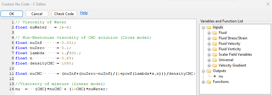
We will use the non-Newtonian viscosity from Benchabane and Bekkour 2008. [1] We present the variation in the protein surrogate viscosity as a function of strain and CMC concentration. At concentrations relevant here, the surrogate is shear-thinning and can be modeled as a Cross fluid. Superimposed on the experimental data is the rheology predicted for a 0.6% surrogate, which is developed using the parameters presented by the authors.
Model Setup
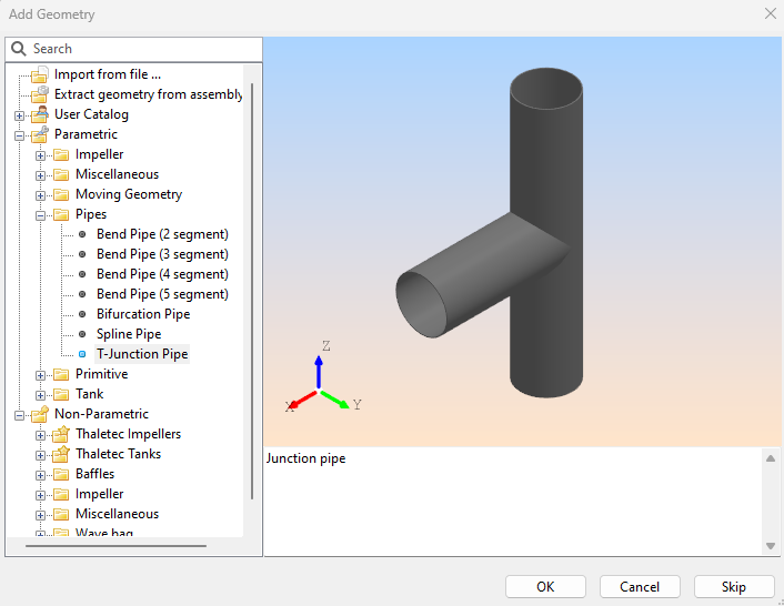
We start by adding a T-junction pipe.
Add a Static Body from Parametric > Pipes and choose the T-Junction Pipe.
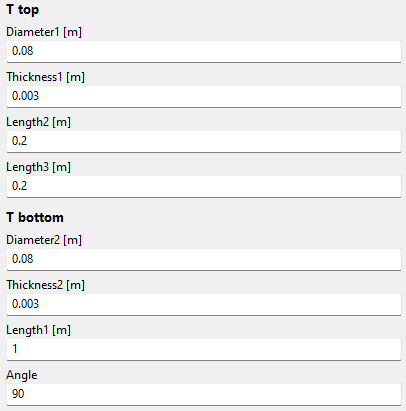
We will change the length of the T bottom to 1 m.
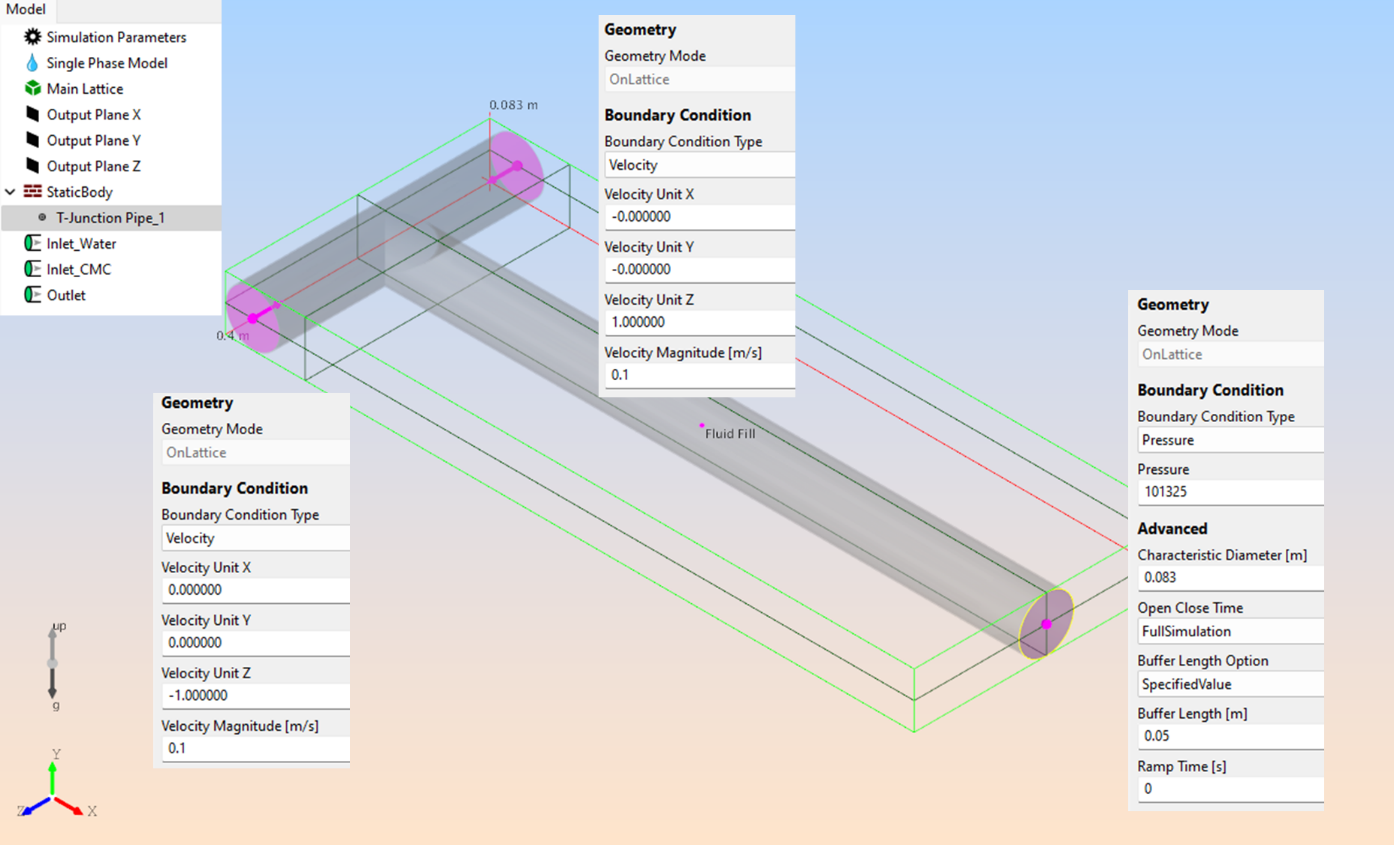
Now let’s add three Boundary Conditions.
Go to Create > Static Inlet/Outlet and select an inlet (select Edges or Point on bounding box). Make sure that the inlets point inward. Rename them to ‘Inlet_Water’, ‘Inlet_CMC’, and Outlet.
Leave the inlets as Velocity Boundary Condition Type and set the Velocity Magnitude [m/s] to 0.1.
For the Outlet Boundary Condition type, select Pressure. Here we want to increase the Buffer Length [m]. This creates a higher viscosity at the pipe outlet, thereby increasing stability. This is often a good idea when you run into instablities at a boundary condition.
The setup should like like this:
Now let’s add the CMC solution.
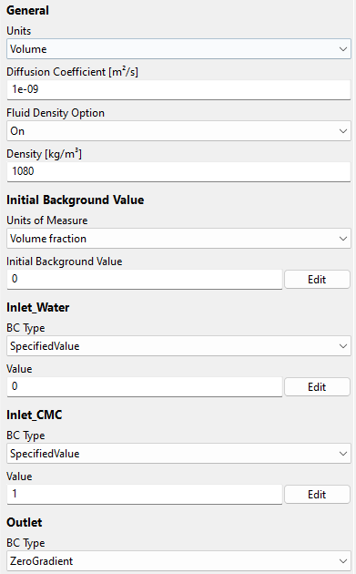
Go to Create > Scalar > Miscible Scalar and skip the geometry selection because we are using an inlet for the addition. Rename it to CMC.
Enable the Fluid Density Option and set the Density [kg/m^3] to 1080.
Change the Inelt/Outlet properties so that the ‘Inlet_CMC’ has a specified value of 1. That means that we are adding the 0.6 % CMC solution at one inlet. The Outlet should be ‘ZeroGradient’.
Implement the non-Newtonian Cross model and a simple mixing law for the viscosities. Change the Rheology Type from ‘Newtonian’ to ‘CustomExpression’ in the Single Phase Model.
Simulation Parameters
Now let’s adjust some settings before running the simulation.
Under ‘Simulation Parameters’ change the Reference to ‘Y’ so we define the resolution across the pipe diameter, and set it to 40. The long section of the T-junction has a higher average velocity magnitude than the two Inlets, so we should reduce the Courant number accordingly. Set the Courant Number to 0.01. A simulation time of 20 seconds should be sufficient.
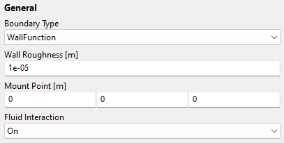
Enable the Turbulence Wall Function in the ‘StaticBody’ properties and define the Wall Roughness [m]. Set it to 1e-5.
The model is now set up, but we can add some additional output and check the influence of a static mixer. We will record the relative standard deviation of the CMC solution in different parts of the pipe.
Start by creating a Global Variable. Rename it to ‘CMC_RSD’ and select Fluid as a Data Source, RelStdDev (%) as Reduction, and use ‘value = CMC;’ as Code. We will now measure the relative standard deviation of the CMC solution. A lower value means better homogenization.
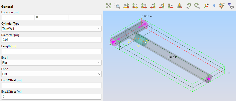
Add geometry to the Global Variable by selecting Parametric > Primitive > Cylinder and rotate it -90° around Z. Change the Diameter to 0.08 and move it to 0.1 m in X-direction.
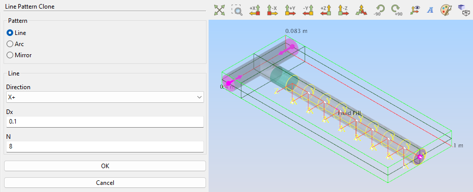
Now select the Global Variable in the model tree, go to Edit > Duplicate Object Pattern, and create eight copies as a line along the X+ direction.
We can now run the simulation.
Additional Output
The rest of the tutorial is not relevant for the purpose of using a custom rheology. However, we can add a static mixing element and compare the results.
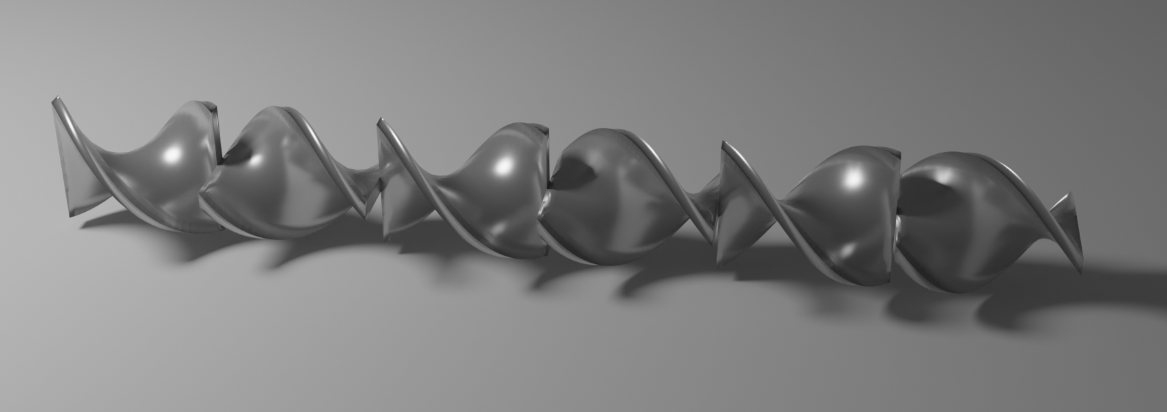
Start by adding a Twist Element to the Static Body (You can create a new static body for that if you want to control the wall treatment for this specific part).
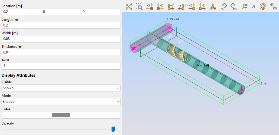
Select Create > Static Body > Add Geometry > Parametric > Miscellaneous > Twist Element.
Rotate it around the Y-axis and use the following settings. Use a different geometry/parameter set at your convenience. Make sure that the Flood Fill Point is not located inside the static part.
Results
The images below are the results of both setups: Without the static mixer (top) and with the static mixer (bottom).
The central bar-plot shows the relative standard deviation of the CMC solution. The bar plot is aligned with the position of the global variables and the static mixer is installed in region 1 and 2.
We can see an interesting effect here. The mixing of the CMC solution is poor before it enters the static mixer. We get two separated streams which cannot mix, so there is one stream with a higher and one stream with a lower concentration.
The blue background indicates the region where the mixing is actually worse for the static mixer. Further downstream, the mixing effect of the rotating flow becomes dominant in the static mixer setup and we see a significant improvement.
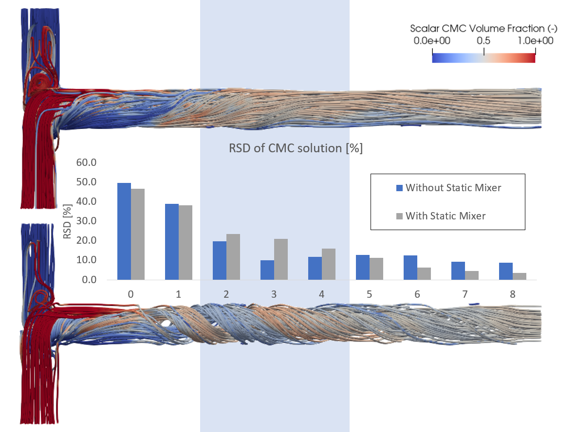
This is why static mixers are usually a series of twist elements that are rotated at a 90° angle so the streams are constantly recombined.