Tutorial for Optimizer: Simple

In this simple case, we will optimize the position of the middle one of three impellers mounted on the same axis to achieve maximum energy input. We are maximizing the power number of the tree impeller system.

First, start by generating a tank geometry:

• Generate a Static Body and choose the Cylindrical Tank.

• Generate a Moving Body and add three Rushton Impellers (Impeller > Parametric > Rushton).

  We use the default 60 RPM here.

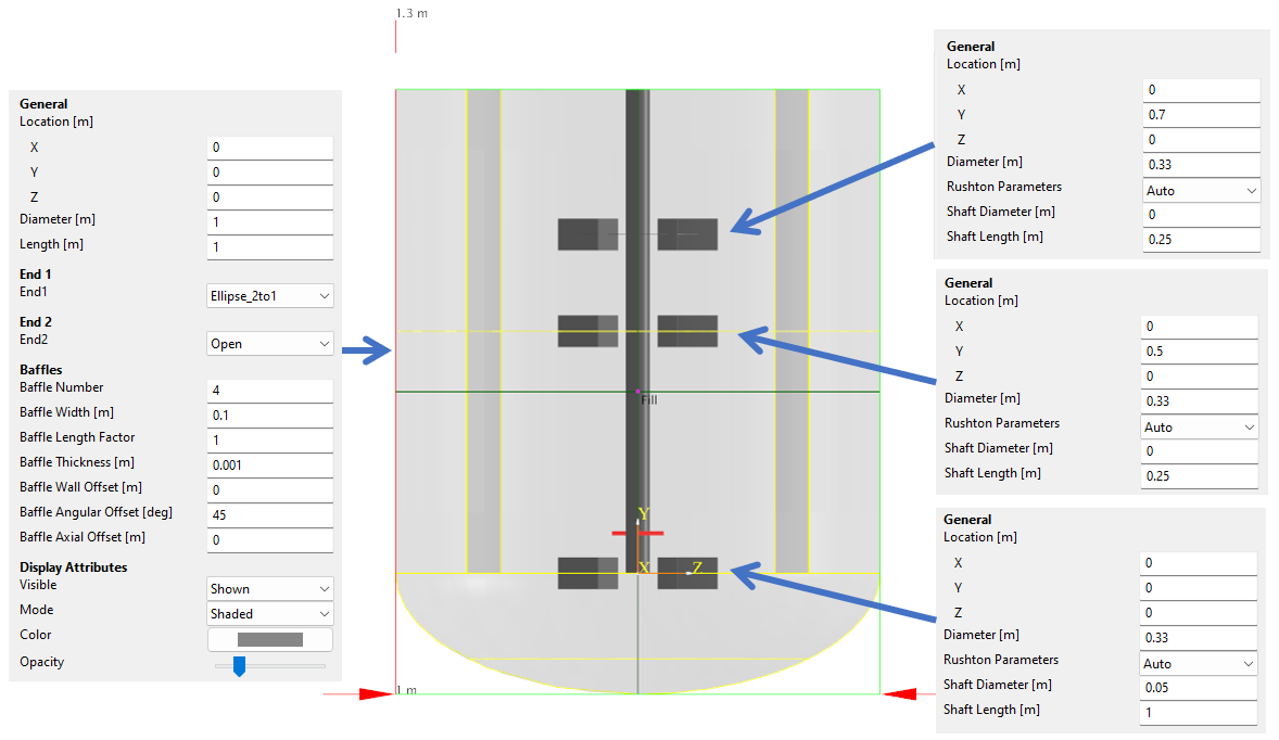
Static Body on the left; Moving Body geometries on the right.

Add two Global Variables:

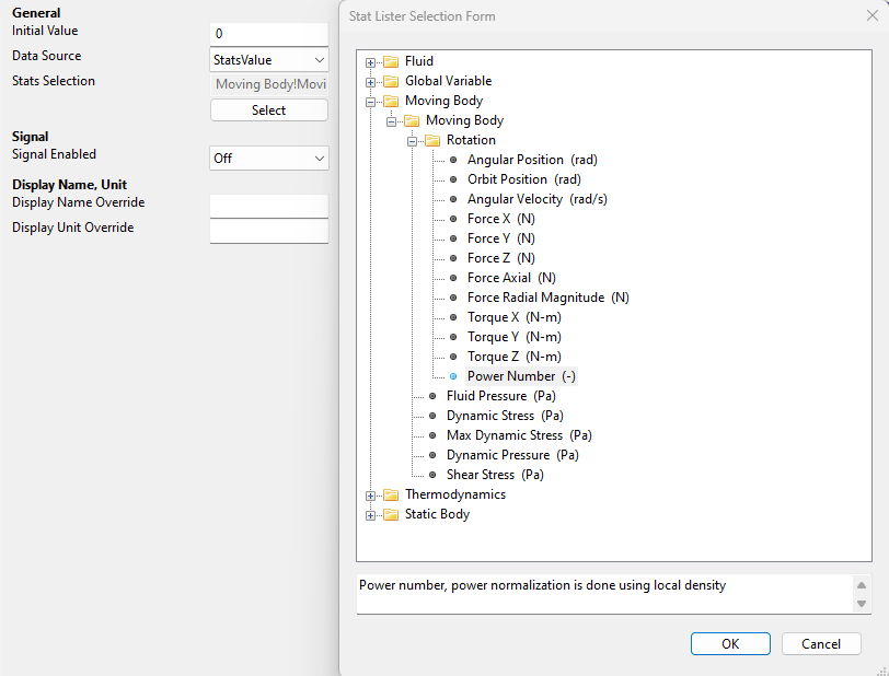
• 1. Name: Po

  On Data Source choose StatsValue and under the Moving Body > Rotation select the Power Number:

  

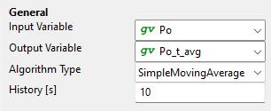
• 2. Name: Po_t_avg

  Leave Data Source as None and the Initial Value as 0.

  Now add an Averaging Filter and smooth out the Power Number over 10 seconds:

  

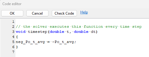
  We want to maximize the time averaged Power Number, but optimizers are minimizers, so we need to minimize a variable. We will simply use the negative time averaged Power Number for that.

Add another Global Variable, leave the default setting (Data Source: None; Initial Value: 0), and call it “neg_Po_t_avg”.

• Add a Custom Script and use it to make the Power Number negative:

  

Now, let’s adjust the maximum Run Time, Resolution and Output Settings.

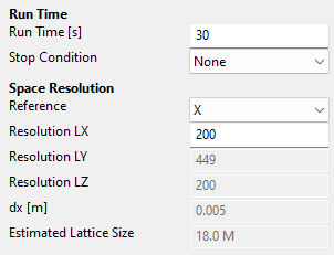
We don’t need a lot of Output because we are more interested in the Global Variables. Let’s increase the frequency for planes to 5 seconds, and for volumes to 99 seconds, so we don’t save any volumetric data.

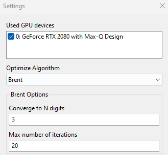
Now, everything is in place to set up the Optimizer. We use 1-D optimization with the Brent algorithm because we only have a single value that we change (y-Position of the middle impeller). See here for more information: https://en.wikipedia.org/wiki/Brent%27s_method

Solve > Run Optimizer and change the Setup:

Now select the Minimized Variable as our Global Variable neg_Po_t_avg and choose the y-position of the middle impeller (Rushton_2):

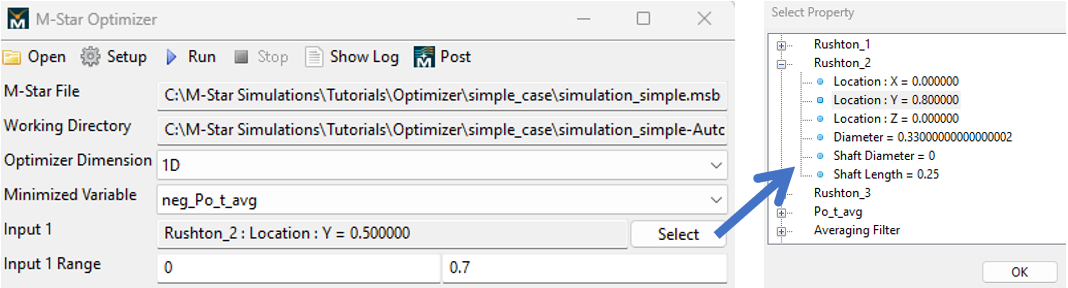
Change the Input Range to 0 and 0.7. This allows the middle impeller at most to overlap with the top or bottom impeller. We assume that only one global minimum exists.

Run

Let’s have a look at the results:

The Optimizer found a converged solution after 10 simulations.

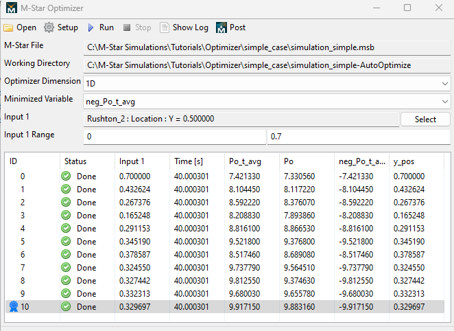
The optimal y-Position is at 0.33 m. The complete Optimization is shown in the following figure. The number denominates the ID and thus the order of the simulation runs. The best position seems to be a bit below the center between the top and bottom impeller indicated by the gray line.

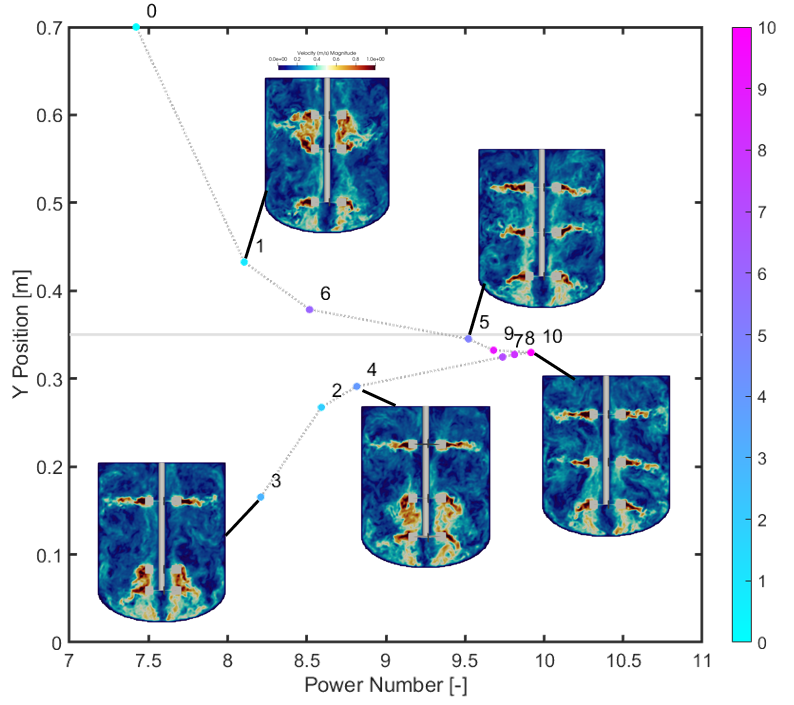
This makes sense because the baffles do not reach down into the curved bottom, allowing a radially circulating flow below the baffles that gets fed by the radial and axial from the bottom impeller. This causes the flow direction from the bottom impeller to have a downwards tilt.