Optimizing Bubble Models: Complex
Overview
This guide demonstrates how to calibrate a bubble breakup and coalescence model using the 2D Optimizer. The objective is to reproduce experimentally measured volumetric mass transfer coefficients ([kLa]) by adjusting empirical parameters in the equilibrium bubble diameter model.
The example uses a parcel-based bubble representation and replaces poorly characterized physical parameters (e.g., surface tension effects in culture media) with empirical coefficients.
Objective
The mass transfer coefficient [kLa] depends on various liquid properties, such as surface tension, salinity, surfactants etc. Typically, culture media are not characterized very well, but the [kLa] can be measured during the process.
In this example, we want to find a model for the [kLa] that reproduces three experimentally measured [kLa]s by using an optimizer in order to adjust the breakup and coalescence model. We will use a parcel approach for the bubble size and adjust the local bubble diameter by replacing the physical parameters with empirical ones, because we don’t have full knowledge of the culture broth.
In this case, we have the following measured values. The sparged gas rate could also be varied, but we are focusing on the impeller speed:
Impeller Speed [RPM] |
[kLa][1/s] |
|---|---|
20 |
0.0009 |
50 |
0.0013 |
70 |
0.0017 |
The setup will sequentially go through the three RPMs, record the difference between simulation and measurement, and minimize this offset.
Model Setup
The vessel is a three-stage Rushton turbine setup. We create a static body with a cylindrical tank and a moving body with three Rushton turbines:
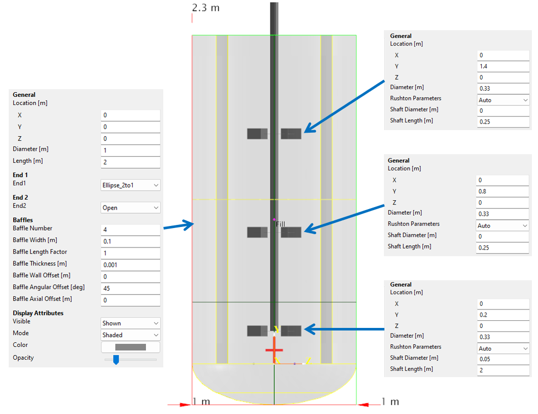
Next we add the bubbles.
We start by adding a Torus (Primitives) as the bubble source:
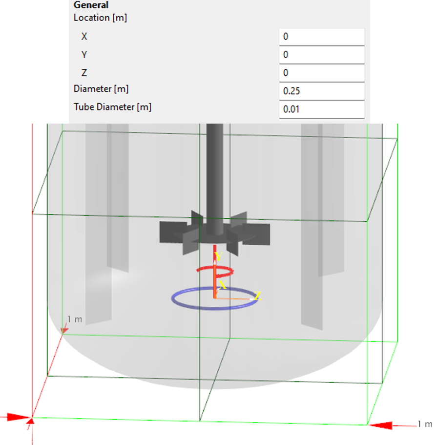
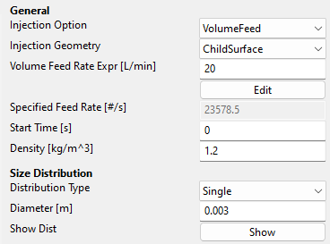
We are sparging 20 liters per minute, and we are setting the initial bubble diameter to 3 mm:
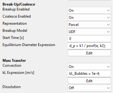
We are leaving the Fluid Interaction and the Static Body Interaction as default and enable breakup and coalescence and choose the parcel representation with our own UDF for the equilibrium diameter.
We are using a constant [kL] expression.
The default equation for the local bubble diameter is
This equilibrium diameter defines the local parameter depending on the local dissipation rate 𝜀 with the material properties surface tension 𝜎 and density 𝜌 which we assume to be global.
We are keeping the general structure of the equilibrium diameter, but we are replacing the unknown parameters with the Global Variables [k1] and [k2] which will be used for model calibration:
This implies that we do not fully understand the physics of the complex culture broth in terms of surface tension, salinity, surfactants, etc., to make predictions about breakup and coalescence behavior.
Simulation Efficiency Adjustments
We have reduced the problem to two unknown variables now, and we can use the 2D Optimizer to find a good match between modeled and measured values.
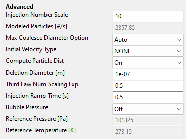
We change the Injection Number Scale to 10 to further reduce the simulation time. We want a very efficient simulation setup, because we are simulating this setup a couple of times.
Global Variables and Constants
We will now add some global variables to the optimizer:
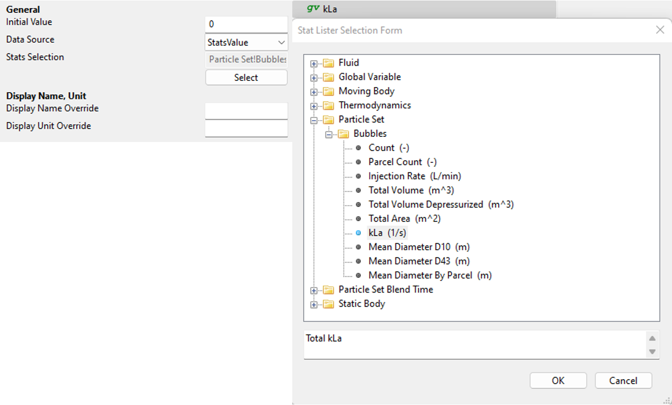
First, we create a Global Variable, call it “kLa”, and extract the [kLa] from the Output Stats data:
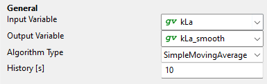
The [kLa] fluctuates, so we want to make the signal smoother. Create a Global Variable called “kLa_smooth” without a data source, and add an Averaging Filter. We average over 10 seconds:
Next we add a Global Constants table:
Global Constant Name
Value
RPM_1
20
RPM_2
50
RPM_3
70
t_RPM_12
30
t_RPM_23
60
Then we add the experimental values, such as Global Variables. We could also add them to the Global Constants, which would be more appropriate; but defining them as Global Variables helps us to check the results and compare between the experiment and simulation quickly. Add the following ones:
Global Constant Name
Value
kLa_exp_1
0.0009
kLa_exp_2
0.0013
kLa_exp_3
0.0017
These are the three experimental [kLa] values and the corresponding impeller speeds, as well as two time points, where we switch the impeller speed.
Finally, we will add 6 more Global Variables that we use for the calculation of the total difference between simulation and experiment and for the Optimizer:
Global Constant Name
Value
difference_1
0
difference_2
0
difference_3
0
total_difference
0
k1
0
k2
0
Note
The global constants difference_1, difference_2 and difference_3 are the differences between the measured and the simulated [kLa] values; total_ difference is the sum of the three; and k1 and k2 are the equilibrium diameter parameters of our bubbles.
Custom Script
Now that we have the infrastructure that we need, we will add a Custom Script. This script calculates the differences which we want to minimize with the optimizer:
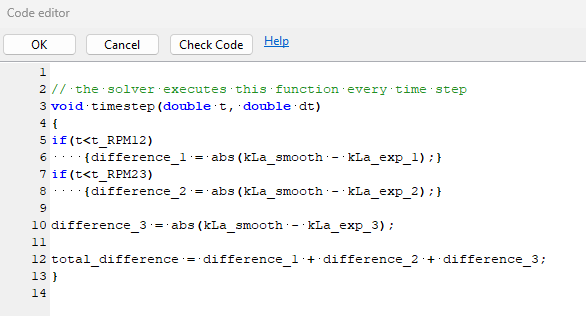
The differences are just the absolute differences between the smoothed [kLa] and the experimental values. We stop to update these differences as we switch to the higher impeller speeds–that means that at the end of the simulation, each experimental [kLa] corresponds to the simulated one at the correct time point. We add up these differences for the optimization (minimization).
We calibrate the timestep to the fastest RPM by setting the impeller speed to 70 RPM and by locking the timestep to this impeller speed. We lock the timestep by changing the Time Step Option from Auto to DtSpecified:
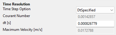
We are not changing the resolution to have fast results. In a real application, the resolution might have to be adjusted to achieve better results.
We are then using the following expression for the Moving Body Rotation Speed [rpm]:
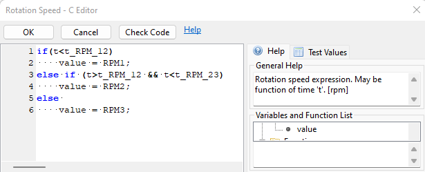
Each run will generate a lot of data by default, so we change the Output Settings. Export the slice data every 10 seconds to get some visual feedback, and set the volumetric output to 999 seconds to not save the data at all.
The impeller speed should be changing over time while we record the [kLa] and compare it to the measured values. The equilibrium diameter of the bubbles is parametrized, which allows us to use it as an input for the optimizer.
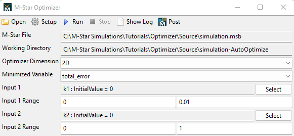
Optimizer Setup
Let us now set up the optimizer and see what happens:
Save the Simulation Setup.
Solve -> Run Optimizer
Open the Setup and select your GPU and the following optimizer setting:
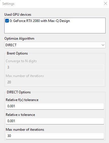
We are choosing small tolerances and 30 runs. That means that all 30 runs should be completed, and the results can then be compared. The DIRECT Optimizer trisects the parameter spacer and repeats for the most promising sector:

For an air-water system, the parameters are: k1 = 0.0023 and k2 = 0.4. We can use these values to set some meaningful boundaries to the parameter space of k1 and k2:
Results
After running the optimizer, we obtain the following results:
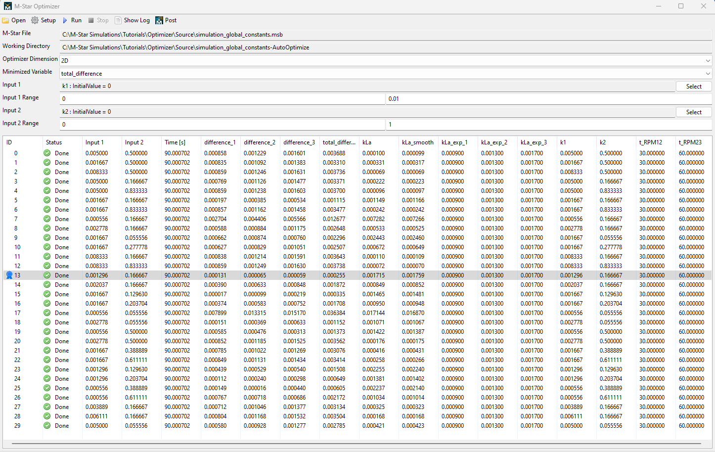
Run 13 seems to be the best one. Let us take a closer look by opening M-Star Post and plotting the Global Variables for the different kLas (This comparison is the reason we defined the experimental kLas as Global Variables):
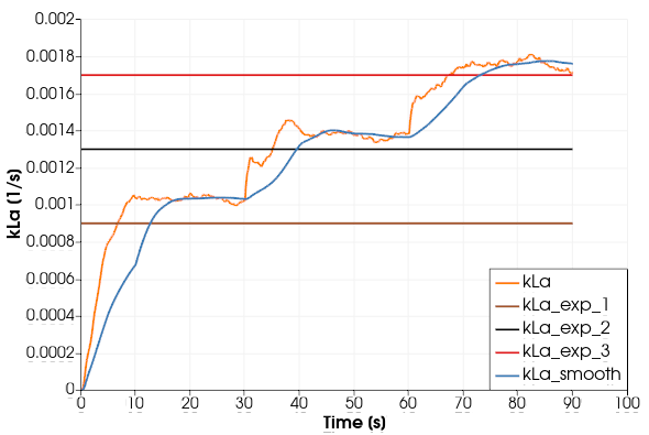
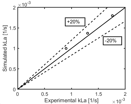
We get very good agreement for this setup. If you want to get a better match, you can do a second optimization sweep with a narrower parameter space for k1 and k2. You can look at other runs to get a sense of the optimization and the sensitivity of the result regarding the input parameters.
This is how the parameter space was sampled by the DIRECT Optimizer.
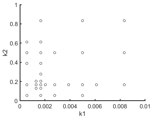
We can see that the optimizer narrows down on the bottom left region where we find our best solution.