Static Inlet Outlet¶

Introduction¶

Static inlets and oulets are boundary conditions through which fluid, particles, species, and energy may enter or exit a system. The fluid entering the system through an inlet can contain a user-defined temperature, user-defined species concentrations, solid particle densities, and bubble volume fractions. Examples of systems with fixed inlets and outlets include openings in a pipe, fluid nozzles, recirculation loops, dip tubes, and drains.

Static inlets and outlets must be defined on a static geometry and exist along the interface of the flood fill volume. The static boundary condition cannot be exposed to the fluid domain on both sides, the flood fill can touch only one side.

Static inlets and outlets can only be defined for single phase, free surface, and two-fluid immiscible fluid configurations. They cannot be defined for background fluid and no-fluid configurations.

Boundary conditions not affixed to a static surface are Moving Inlets and Outlets.

Whenever a static inlet or outlet is added, the user is prompted to the Inlet/Outlet Setup form. Here users have three options for defining the position of a static inlet or outlet: (1) select an existing surface along a static body; (2) select an existing edge of a static body to define a new surface; or (3) select a point on the bounding box surface. For a tutorial illustrating all three methods, see selecting surfaces for boundary conditions.

Various conditions can be specified along the surface of the boundary condition, including user-specified velocity, pressure, volumetric flow rate, and mass flow rate. Static inlets and outlets can be linked to other boundary conditions via a recirculation coupling. All boundary conditions assigned to a static inlet or outlet can also vary in space (along the boundary condition surface) or time.

Systems may contain multiple boundary conditions. For single-fluid systems, the system should contain at least one inlet and one outlet. Since the fluid volume is constant in these systems, inflow must be balanced with outflow. Simulations with filling and draining systems, as modeled using a free surface model, need only one boundary condition. These points are discussed in the pipe flow and tank filling/draining tutorials.

Property Grid¶

`Boundary Condition`¶

Boundary Condition Type

There are ten options for defining inlet and outlet boundary conditions:

Pressure: Specified pressure along the surface of the boundary condition. Value may be time-dependent.
Velocity: Specified velocity along the boundary condition surface. Velocity vector along the boundary condition surface may vary in space and time.
Outflow: Zero-velocity gradient in the direction normal to the surface.
Recirculation Return: Boundary condition that is coupled to another boundary condition in the system. Used to model recirculating systems.
Poiseuille: Fully developed laminar velocity profile.
Volume Flow Rate: Volumetric flow rate along the boundary condition surface. Value may be time-dependent.
Mass Flow Rate: Specified mass flow rate along the boundary condition surface. Value may be time-dependent.
Inlet Single Pulse: Single pulse of fluid added at a set time with a specified velocity, volumetric flow rate, or mass flow rate.
Inlet Multi Pulse: Periodic set of pulses with a user-specified velocity, volumetric flow rate, or mass flow rate.
Pump Curve Intake: User-imported pumping curve which links flow rate to pressure differences.

`Reference`¶

Geometry Mode (READ ONLY)

This mode describes the orientation of the boundary condition surface relative to the underlying fluid lattice.

On Lattice: The boundary condition surface is aligned with the X, Y, or Z direction of the lattice.
Off Lattice: The boundary condition surface is skew or not aligned with the underlying lattice.

Note

In general, ‘On Lattice’ conditions are more stable (i.e. more direct, less interpolated, less likely to crash). If possible, efforts should be made to make boundary conditions on lattice. For a tutorial, see On and Off Lattice Boundary Conditions.

Point

m | The reference point for the inlet/outlet. This is the user-defined point that will be the seed for the two-dimensional flood fill along the selected bounding box surface. This location/seed point also acts as the origin for spatially varying boundary conditions (e.g., fluid type, velocity, temperature, species concentration) along the boundary condition surface. For inlets and outlets defined using surfaces or edges, this is the centroid of the boundary condition surface. It is computed automatically. This point is referenced when defining spatially-varying inlet velocity vectors. See Velocity Unit Vector expressions. specified value

Characteristic Diameter

m | Equivalent hydraulic diameter. This diameter characterizes the extent of the boundary condition. It is used to estimate the computed velocity. The conversion is performed by dividing the user-defined mass or volumetric flow rate by the area calculated from the hydraulic diameter. This computed velocity is then used to set an appropriate simulation time step.

For boundary conditions defined from edges and surfaces, the characteristic diameter is automatically calculated from four times the ratio of the boundary condition area divided by the boundary condition perimeter. This value is presented only as a non-editable reference, confirming to the user that the extent of the boundary condition defined by the GUI is in line with physical expectations. The hydraulic diameter is not referenced by the code when working with velocity and/or pressure boundary conditions, which are used to compute the time step directly.

For boundary conditions defined from a point on the bounding box, the characteristic diameter can be set by the user. This value is not referenced by the code when working with velocity and/or pressure boundary conditions, which are used to compute the time step directly. It becomes important, however, when defining mass or volumetric flow rate boundary conditions.

An improperly specified characteristic diameter will lead to an improper estimate of boundary condition velocity, which will then lead to an improper simulation time step.

Note

For circular boundary conditions, hydraulic diameter reduces to the circle diameter.

Computed Velocity: m/s | Characteristic velocity of the boundary condition. This value characterizes the speed of the fluid along the boundary condition surfaces. For velocity boundary conditions, this computed velocity is equal to the user-defined value. For volumetric or mass flow boundary conditions, this velocity is computed by dividing the user-defined mass or volumetric flow rate by the area calculated from the hydraulic diameter. For pressure and outflow boundary conditions, the computed velocity defaults to 1 m/s. This value is incorporated into the time step calculation.

Note

For systems with constrictions, the realized velocity may exceed the inlet velocity. Attention should be given to the Courant number, as discussed in this tutorial guide.

This section will launch if you select an edge or a surface for the static inlet/outlet

`Display Attributes`¶

Visible

The ability to show or hide the object.

Shown: The object is shown in the 3D view.
Hidden: The object is hidden in the 3D view.

Mode

This offers two options to view the object.

Wire

The object is shown as a wire frame.

Width: The width of the line used to render the object in the 3D view.

Shaded

The object is shown as a shaded surface.

Material: This allows the user to change the material of the object with the following options: Aluminum, Steel, Chrome, Plastic, or Glass.
Opacity: This scale allows the user to change the opacity of the object.

Color

This offers to change the color of the object.

`Advanced`¶

Duration Option

This defines the time interval over which the inlet or outlet boundary conditions are applied. Throughout the specified duration, transport along the boundary condition surface evolves according to the user-defined parameterization. Outside this duration, the velocity along the boundary condition surface is set to zero. This change is analogous to closing a valve in a system, meaning there is no mass, species, momentum, particle, or thermal transport across the boundary condition surface. This behavior overwrites all user-defined parameters and sets the velocity/fluxes to zero.

Full Simulation

Transport along the boundary condition surface evolves over the entire simulation.

Single Interval

Transport along the boundary condition surface evolves over the duration specified by the start and end time. Outside this interval, the velocity along the boundary condition surface is set to zero.

Start Time: Start time for transport along the boundary condition.
End Time: End time for transport along the boundary condition.

Custom Expression

Transport along the boundary condition surface evolves over a custom user-defined expression. When the expression output is set to zero, there is no mass, species, momentum, particle, or thermal transport across the boundary condition surface. When the duration is set to one, the velocity along the boundary condition surface evolves according to the user-defined parameterization.

Open Close UDF: unitless | This UDF is an expression for the open close condition. An output value greater than zero is interpreted as an open condition, and less than zero is interpreted as a closed condition. This is a System UDF.

Download Sample File: Open Close

Buffer Length Option

m | The options to modify buffer length for inlet and outlet conditions in model units. In systems with large openings, the flow field interacting with the opening may be complex, and a buffer may be required to maintain overall stability. A buffer is a region near the inlet/outlet wherein the fluid viscosity is artificially inflated to decrease small-scale variations in the flow field. The net effect is to one-dimensionalize the flow at the boundary condition surface. Reducing cross-sectional variations helps to maintain stability. For systems with inlet/outlet diameters that are small compared to the tank diameter, flow through the orifice is typically one-dimensional and boundary conditions are generally stable.

Buffers are typically applied to boundary conditions where the velocity is not specified (e.g., pressure, outflow, etc.). The buffer does not affect mass continuity, but the additional viscosity introduced by the buffer will increase local pressure drop. To minimize its effects on flow, the buffer should be made as small as possible. The buffer can be visualized in M-Star Post by rendering the Effective Viscosity in the Volume View.

Auto

The buffer extends one lattice point in the direction normal to the boundary condition surface.

Specified Value

User-specified buffer length. To prevent excessive perturbation to the local fluid dynamics, the maximum buffer length should not exceed the diameter of the inlet. See the buffer length tutorial.

Buffer Length

m | The thickness of the viscosity buffer in the direction normal to the boundary condition surface.

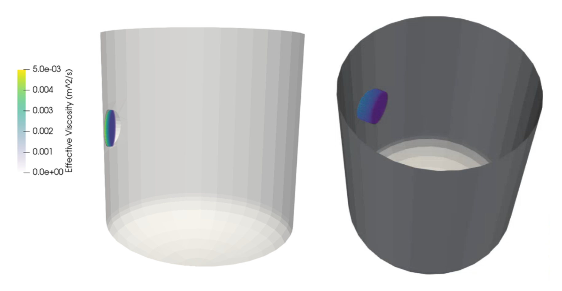
These tanks show two examples of buffer length. The left tank has a fairly thin buffer, while the right tank has a thick buffer (note that the length does not exceed the diameter of the inlet).

Ramp Time

s | Ramp time for boundary condition.

For constant velocity boundary conditions, this is the interval over which inlet velocity will be increased from zero to the user-defined constant velocity, via a quarter sine wave.

For constant pressure boundary conditions, this is the interval over which the inlet pressure will be increased from the initial fluid pressure to the user-defined constant inlet pressure, via a quarter sine wave.

Mathematically speaking, the ramp prevents the system from realizing an infinite acceleration at the boundary condition over the first time step. Physically speaking, the ramp is analogous to the time required to open a value and actuate a pump.

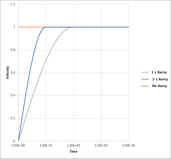
../../../_images/ramp-time.png — This graph shows an example of a zero, half-second, and one-second ramp time with a steady-state velocity of one meter per second.¶

Note

The purpose of the ramp is to limit the propagation of “shock waves” throughout the system, associated with a step-increase in boundary velocity or pressure.
The duration of the ramp time, in terms of time steps, should be comparable to the number of lattice points across the system domain.

Pressure Filter

The pressure filter is used to attenuate spurious pressure waves. These waves commonly occur in systems that have sudden changes in boundary conditions, free surface dynamics, or other physics thereby causing pressure oscillations. This advanced feature is discussed further in a tutorial.

Off

No pressure filter applied.

On

A time-constant parameter is engaged which is typically set to a duration equal to a few periods of the observed pressure waves.

Pressure Filter Time Constant: s | The timescale over which the time averaging happens.