Immiscible Two Fluid¶

Introduction¶

Immiscible two fluid configurations involve two immiscible fluids with Newtonian or non-Newtonian rheology and the dynamic interface between the fluids. These models use a volume-of-fluid approach to define the interface between the two fluids, which is modeled explicitly. Users must specify for each fluid the density and the constitutive relationship between fluid stress and fluid strain. Fluid dynamics in both fluids are modeled explicitly via the Navier-Stokes equations. Users must also specify a surface tension between the two fluids. This configuration can also support species transport across the two-fluid interface, as well as particle transport/trapping within and between fluids. If transport in one of the two fluids is irrelevant, as may be realized in systems with high fluid density ratios, apply a free-surface configuration.

Conceptually speaking, the two fluids in the simulation domain are expressed by tuning the background fluid, setting the properties of the child geometry attached to the fluid, and adding initial condition fill points to the simulation. The background fluid represents the initial fluid filling the domain. The child and fill points define where the second fluid initially exists. Fluids can also enter the system via inlets and outlets, as well as via particle-fluid conversion. These points are discussed below.

Common applications include two-phase gas flow simulations, colloid suspensions, and oil-water systems.

The context-specific immiscible two fluid toolbar can be used to add children geometry, as well as move, rotate, and/or scale all the child geometry attached to the fluid parent. In addition to these operations related to child geometry, options are presented for adding child fill points and editing inlet/outlet boundary condition tables.

For convenience, a fluid height box child geometry is added to the system when setting up an Immiscible Two Fluid configuration. This child geometry can be deleted, modified, or combined with other child geometry to match the required initial conditions.

Property Grid¶

The immiscible two fluid property grid is unique based on your fluid setup and fluid rheology.

`Fluid Properties`¶

There are two ways to define the fluid setup for immiscible two fluids. The first is to define the rheologies independently using the Separate Rheology set up. Select from the predefined rheology sets and define the density and parameterization. The second way is to use the Combined Rheology expression wherein you define the density of each fluid and a custom expression for the fluid viscosity.

Fluid Setup

The fluid properties of this configuration depend upon the rheology.

Separate Rheology: Two individual rheologies combined by applying simple volume averaging.
Combined Rheology: User defines an expression for viscosity.

Fluid 1 Name

Optional text field to provide a name for Fluid 1 (e.g., “air,” “water,” “oil”). This name will propagate throughout the GUI and output files.

Fluid 2 Name

Optional text field to provide a name for Fluid 2 (e.g., “air,” “water,” “oil”). This name will propagate throughout the GUI and output files.

`Fluid 1 Rheology`¶

Select the rheology type from the available list to show the accompanying grid—this type is listed on each grid as Fluid 1. Fluid 1 should be the lower volume fluid.

Rheology Type

Newtonian: A fluid with a constant and uniform viscosity.
Power-law: Local fluid viscosity is calculated from the local shear rate using a user-defined flow consistency index, flow behavior index, and yield stress.
Carreau: Local fluid viscosity is calculated from the local shear rate using a user-defined characteristic time, power index, and infinite/zero share rate viscosities.
Cross: Local fluid viscosity is calculated from the local shear rate using a user-defined rate constant, time constant, and infinite/zero share rate viscosities.
Bingham Plastic: A viscoelastic fluid with a user-defined yield-stress and viscosity.

`Fluid 2 Rheology`¶

When two fluid rheologies are selected, the property grid configuration will default to the rheology with the maximum number of components.

Rheology Type

Newtonian: A fluid with a constant and uniform viscosity.
Power-law: Local fluid viscosity is calculated from the local shear rate using a user-defined flow consistency index, flow behavior index, and yield stress.
Carreau: Local fluid viscosity is calculated from the local shear rate using a user-defined characteristic time, power index, and infinite/zero share rate viscosities.
Cross: Local fluid viscosity is calculated from the local shear rate using a user-defined rate constant, time constant, and infinite/zero share rate viscosities.
Bingham Plastic: A viscoelastic fluid with a user-defined yield-stress and viscosity.

If Combined Rheology is selected, the following section will launch:

`Combined Rheology`¶

Here you enter the density of each fluid independently as well as a user-defined function explaining how the density varies as a function of the volume fraction of each fluid.

Density1

kg/m ³ | The density of Fluid 1.

Density2

kg/m ³ | The density of Fluid 2.

Kinematic Viscosity UDF

m ² /s | This UDF defines the fluid’s local viscosity. It requires a single output: a floating-point variable named nu, which represents the local viscosity of the fluid. This is a voxel-based local UDF, calculated on a voxel-by-voxel basis using the local fluid properties.

Download Sample File: Kinematic Viscosity

`Configuration`¶

These properties define the configuration of the fluid, including the turbulence type and any external acceleration.

Initial Fluid Pressure

Pa | Initial pressure of the fluid inside the system.

Turbulence Model Type

Fluid turbulence model to be applied to the simulation.

DNS

These simulations attempt to capture all fluid motion across all eddy scales. DNS simulations will diverge if the eddy size approaches the lattice spacing.

LES

These models compute a local eddy viscosity using the local shear rate to capture the effects of sub-grid turbulence. This eddy viscosity is then superimposed on the molecular viscosity when solving the Navier-Stokes equations. LES models tend to be stable at arbitrary Reynolds numbers. The effects of the filter on fluid flow decrease with increasing resolution.

Smagorinsky Coefficient: Only relevant for LES simulation. This value is set to 0.1, a value motivated by predictions from direct numerical simulation.

ILES

These models use a larger (27-vector) lattice stencil and a cumulant-based momentum integrator to maintain stability at higher Reynolds numbers. No modification to the viscosity. ILES may be superior for systems with very low Reynolds numbers.

Lattice Type

This setting defines the number of discrete microscopic velocity vectors considered at each lattice point. The D3Q19 and D3Q27 lattice models differ primarily in the number of discrete velocity directions. The D3Q19 model has 19 possible velocity directions, while the D3Q27 model has 27. The additional directions in the D3Q27 lattice allow it to capture more complex flow details, particularly in simulations involving higher Reynolds numbers or intricate boundary interactions.

However, this increased complexity comes at a cost: the D3Q27 model typically requires about 40% more memory and runs about 40% slower than the D3Q19 model, making it more computationally demanding. When choosing between them, consider the trade-off between accuracy and computational efficiency. D3Q27 may be preferred for simulations which require high precision in flow characteristics, whereas D3Q19 may be preferable when the priority is computational efficiency.

D3Q19: Uses a D3Q19 lattice.
D3Q27: Uses a D3Q27 lattice.

Note

These options are only available for DNS and LES Turbulence Model Types. The ILES Turbulence Model requires a D3Q27 lattice and is set automatically by the solver at runtime.

High Density Ratio

Enable high density ratio algorithm. This is recommended for any system where the density ratio exceeds 2:1.

Off: No high density ratio algorithm.
On: Enables high density ratio algorithm.

Enable Surface Tension

Surface tension of the fluid in the gas.

Off: No surface tension is enabled.
On: Enables surface tension of the fluid in the gas.

Surface Tension

N/m | Surface tension of the gas/liquid interface.

Particle Trapping

If enabled for Fluid 1 or Fluid 2, this option will trap particles within a given fluid.

Disabled: No particle trapping in either fluid.
Fluid1: Traps particles in Fluid 1.
Fluid2: Traps particles in Fluid 2.

Enforce Conservation

This option activates an algorithm to correct any conservation error. Because the scalar advection algorithm is not conservative near the free surface, the scalar field throughout the system is adjusted so that the total amount of scalar matches the initial amount plus or minus any injection or removal.

Off: Algorithm deactivated.
On: Activates algorithm to correct conservation error.

Enable Evaporation

This option can be used to model mass loss across the two-fluid interface. Enabling this feature will cause the fluid volume in the evaporating phase to decrease according to a volume transfer rate UDF.

Download Sample File: Enable Evaporation UDF

Off

No mass transfer across the interface

On

Calculates mass transfer across the interface.

Evaporation Expression UDF: m³ /s | This UDF defines the evaporation rate at the interface. Positive values add fluid and negative values remove fluid. This transfer rate is applied uniformly across the fluid interface. The evaporating fluid is identified by the Evaporating Fluid selection (below). This is a System UDF.
Evaporating Fluid: Defines which fluid is evaporating, Fluid 1 or Fluid 2.

VOF-Moving Body Interaction

This option will apply additional forcing to prevent the multiphase interface from penetrating a moving body. Due to the nature of the immersed boundary method used for moving bodies, fluid can leak through these geometries over the course of a simulation. This is particularly undesirable when one phase in a multiphase simulation needs to be contained within a moving body. The magnitude of this parameters controls the magnitude of the forcing applied; increase or decrease as needed.

Off

No additional forcing applied to prevent penetration.

On

Additional forcing applied to prevent penetration.

Vof Ibm Normal Force Value: Additional force value applied to prevent penetration.

`Interfacial Scalar Transfer`¶

Scalar transfer can be used to model species transfer across the interface between the two immiscible fluids. This functionality is particularly useful when modeling gas transfer/stripping in multiphase systems and droplet curing processes in liquid/liquid dispersions. The transfer model requires a unique scalar field for the species in each liquid. Users must define a scalar field representing the species concentration in Fluid 1 and a second scalar field representing the species concentration in Fluid 2. Users must also provide a framework describing transfer between the two species across the interface. This framework is a user-defined function that is typically patterned after empirical mass transfer models.

Importantly, the scalar fields participating in interfacial scalar transfer must be contained in each respective fluid.

Note

The transfer model follows a low concentration approximation, meaning the exchange of species across the interface does not affect the volume of each fluid.

In the video and associated input file below, we illustrate this setup for a two-fluid gas/liquid system with interfacial oxygen transfer.

Download Sample File: Scalar Transfer

Enable

Enable scalar transfer. This can be used to model species transfer across the interface between two immiscible fluids.

On

Enable Scalar transfer between the two fluids.

Scalar 1

The first scalar field participating in interfacial transport.

Scalar 2

The second scalar field participating in interfacial transport.

Interface Species Transfer UDF

mol/(m ² \(\cdot\) s), g/(m ² \(\cdot\) s), or m/s | This UDF defines the local scalar flux across the immiscible fluid interface. One output must be defined within the UDF: a floating point variable named flux. The scalar will be reduced in one phase and increased by the same amount in the other phase. Positive values imply flux from Species 1 to Species 2. Negative values imply flux from Species 2 to Species 1.

Both Species 1 and Species 2 have the same base units. The units on the flux variable will be either mol/(m ² \(\cdot\) s), g/(m ² \(\cdot\) s), or m/s, depending on the Base Units. This is a voxel-based local UDF, calculated on a voxel-by-voxel basis using the local fluid properties. The UDF is only applied to cells along the two-fluid interface.

Download Sample File: Interface Species Transfer

Tip

These mass transfer physics are analogous to those used when modeling particle-scalar coupling. The difference is that bubbles/droplets in the two-fluid immiscible model discussed here are explicitly resolved using continuous phase Eulerian representations for both fluids. When using particle-based representations, the bubble/droplets are modeled as Lagrangian spheres moving through a continuous phase Eulerian fluid.

`Initial Condition`¶

By default in an immiscible two fluid model, the initial condition of the simulation domain is set as Fluid 1, and a fluid height box is automatically added as a child geometry with the fluid inside set as Fluid 2. This is how the two fluids are expressed.

Users must specify which portions of the interior zone (if any) are initially filled with each fluid. The child geometry fluid overwrites the background condition with a secondary fluid.

Users specify this initial configuration by either (1) setting the initial condition default, (2) adding child geometry to the two-fluid parent, or (3) adding fill points to the two-fluid parent. Fills points are described in detail below.

Initial Condition Default

The default value for the simulation domain. This setting defines the initial background fluid, which characterizes density and viscosity of the fluid for any points not affected by any subsequent child geometry or fill points. The default is set to Fluid 1, although users can change the initial condition default to Fluid 2.

Fluid1: The initial condition default for Fluid 1.
Fluid2: The initial condition default for Fluid 2.

Enable Fill Volume

Sets the initial fluid level using a user-defined initial fill volume. The process mimics filling a vessel from the top with a specific volume of fluid: the filling starts at the bottommost region(s) of the interior zones and extends upward (in the direction opposite gravity). Since the algorithm uses the results of the flood fill, it automatically respects the contours and topology of the vessel surface.

On

Uses enable fill volume.

Fill Volume: m ³ | Target fluid volume realized during the fill process. Child volumes will overwrite any fill volumes.

Off

Does not use enable fill volume.

Note

This fill volume will be overwritten by any child geometry initial conditions.

`Child Geometry Initial Conditions`¶

Child geometry can be added to the immiscible two fluid parent via the Add Geometry form on the context-specific toolbar. For each child geometry added to the two-fluid parent, users independently specify which fluid (Fluid 1 or Fluid 2) will occupy which child geometry.

As a convenience feature, we preload the Immiscible Two Fluid model with a child geometry fluid height box. This box can be set to Fluid 1 or Fluid 2, just as all other fluid geometry have the same option. It can be deleted or additional geometry can be superimposed upon it.

Fluid Height Box Condition

By default, a fluid height box is anchored to the main lattice domain aligned with the Up direction. The height is automatically one third the domain height. This child geometry launches a unique Fluid Height Box Toolbar.

Fluid1: The default fluid height box for Fluid 1.
Fluid2: The default fluid height box for Fluid 2.

Additional child geometry conditions are listed accordingly (i.e., “Child Geometry Name” Condition).

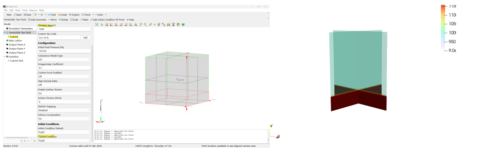
The two-fluid parent can contain multiple children geometry, which can create complex initiation conditions. In the example below, the Initial Condition Default is set to Fluid 1 and the cuboid child geometry is set to Fluid 2. For illustration purposes, the density of Fluid 1 is set to 1000 kg/m3 and the density of Fluid 2 is set to 1200 kg/m3. The resulting initial condition is a stratified system, with an immiscible oil on the bottom of a water-filled vessel

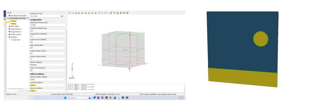
In the next example, the Initial Condition Default is set to Fluid 1, and two child geometry are set to Fluid 2. The resulting initial condition is shown. This configuration represents adding a droplet of oil into a water-filled vessel containing a layer of oil on the bottom.

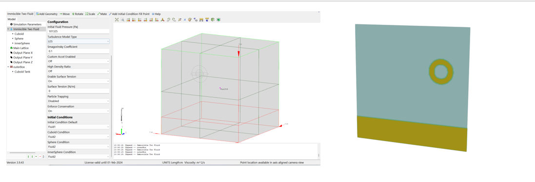
In the example below, we add a third child geometry to the system, which is positioned inside the second child geometry and set to Fluid 1. Note that the order of the child geometry informs the initial structure of the fluid. This configuration represents adding a heterogenous water-in-oil-in-water droplet into a water-filled vessel containing a layer of oil on the bottom.

If fill points are defined, the following section will launch:

`Fill Point Initial Conditions`¶

When static bodies are present, users can specify which fluids occupy the static bodies or the interior via the Add Child Fill Point form. This advanced option is particularly useful for modeling two-fluid heat exchangers wherein the two simulation fluids have different properties but never touch.

Point Condition

Point defines a 3D flood fill to the boundaries of the geometry in which it is contained.

Fluid 1: The fill point denotes Fluid 1.
Fluid 2: The fill point denotes Fluid 2.

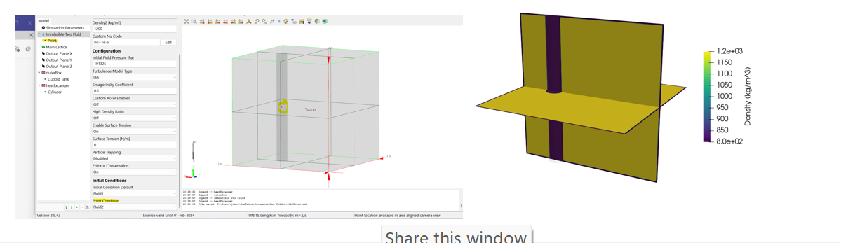
In the example below, a static body named heatExchanger is added to the simulation domain. A fill point is added to the system and placed inside the child geometry. The result is an initial condition where Fluid 2 fills the interior of the child geometry and Fluid 1 fills the vessel. The presence of the static geometry will prevent the two fluids from touching directly.

If a static inlet or outlet is defined, the following section will launch:

`{Static Inlet Outlet}`¶

This defines which fluid is entering the system through each inlet and outlet. For immiscible two fluid simulations, this can be either Fluid 1 or Fluid 2. A row is added for each inlet/outlet defined in the model tree.

Other boundary conditions are defined separately with their respective families, including fluid, scalar field, miscible scalar, free surface volume fraction, thermal, and particle boundary conditions.

Boundary Condition Type

This setting determines which boundary condition will be applied along the inlet/outlet surface.

Specified Value

The specified value launches the user-defined function.

Static Inlet Fluid Type UDF

unitless | This UDF defines the fluid type boundary condition. A value of 1 indicates fluid1 and a value of 0 indicates fluid2. This may be an expression of the form f(x,y,z,t), where x,y,z are positions relative to the inlet seed point and in the Si unit system. The orientation of this local basis set is illustrated in the view panel. This condition is particularly useful when defining partially filled inlets, as illustrated in the example below. This is a System UDF.

Download Sample File: Stratified Fluid

Zero Gradient

A zero gradient boundary condition is applied to the fluid volume fraction. Appropriate for simulations with covered inlets/outlets.

Fluid 1

The volume fraction at the inlet/outlet is 1 for Fluid 1.

Fluid 2

The volume fraction at the inlet/outlet is 1 for Fluid 2.

The Drip boundary condition is used for low-velocity, gravity-driven inlets, typically located in the upper portions of vessels. This prevents fluid leakage that can occur with the Fluid 1/2 boundary condition.

Fluid 1 Drip

Fluid volume fraction for Fluid 1 is maintained at 1 throughout the simulation.

Fluid 2 Drip

Fluid volume fraction for Fluid 1 is maintained at 2 throughout the simulation.

If a moving inlet/outlet is defined, the following section will launch:

`{Moving Inlet Outlet}`¶

Moving Inlet Fluid Type UDF

unitless | This UDF defines a fluid type boundary condition with a moving inlet. A value of 1 indicates fluid 1 and a value of 0 indicates fluid 2. The fluid type is applied across the moving inlet surface. This is a System UDF.

Download Sample File: Moving Inlet Fluid Type

If particles are defined, the following section will launch:

`Fluid Particle Convert`¶

The fluid-particle conversion (a.k.a. Eularian-Lagrangian conversion) algorithm can be used to convert portions of the continuous fluid into discrete particles and/or convert discrete particles into a region of continuous fluid.

The continuous-to-discrete conversion is useful when describing physics such as jet break-up, bubble break-up, and immiscible fluid dispersion processes, wherein initially continuous fluid structures may decompose into structures that are smaller than the grid resolution of the continuous phase fluid.

The discrete-to-continuous conversion is useful when describing physics such as agglomeration, coalescence, droplet simulations, and so forth, wherein initially discrete fluid particles may aggregate and coalesce into structures which are larger than the grid resolution of the continuous phase fluid.

Download Sample File: Fluid Particle Convert

Option¶

This feature allows you to convert either phase of the free surface model into discrete Langrangian molecules.

Off

Algorithm disabled.

Auto

Algorithm active.

Particle Set

Identifies the particle set that will participate in fluid-particle conversion.

Massless Tracers

Inertial Particles

Phase

This is the continuous phase that will be converted into the selected particle set.

Fluid 1: Convert fluid 1 into droplets with the properties defined on the particle set.
Fluid 2: Convert fluid 2 into bubbles properties defined on the particle set.

Start Time

s | This is the time to begin conversion.

Convert Fluid to Particles

This setting controls the direction of conversion. If active, continuous (Eularian) fluid structures will convert into discrete (Lagrangian) particles.

Off: Algorithm disabled.
On: Algorithm active.

Convert Particles to Fluid

This setting controls the direction of conversion. If active, discrete (Lagrangian) particles will convert into continuous (Eularian) fluid structures.

Off: Algorithm disabled.
On: Algorithm active.

Custom

Custom algorithm enabled.

Particle Set

Identifies the particle set that will participate in fluid-particle conversion.

Massless Tracers

Inertial Particles

Phase

This is the continuous phase that will be converted into the selected particle set.

Fluid 1: Convert fluid 1 into droplets with the properties defined on the particle set.
Fluid 2: Convert fluid 2 into bubbles properties defined on the particle set.

Start Time

s | This is the time to begin conversion.

Convert Fluid to Particles

This setting controls the direction of conversion. If active, continuous (Eularian) fluid structures will convert into discrete (Lagrangian) particles.

Off: Algorithm disabled.
On: Algorithm active.

Convert Particles to Fluid

This setting controls the direction of conversion. If active, discrete (Lagrangian) particles will convert into continuous (Eularian) fluid structures.

Off: Algorithm disabled.
On: Algorithm active.

Particle to Fluid Diameter Cutoff

m | Discrete (Lagrangian) particles with diameters larger than this value will convert into a continuous (Eularian) fluid structure.

Particle Immersion Cutoff

Discrete (Lagrangian) particles will be absorbed into the continuous (Eularian) fluid at this volume fraction cut-off

Fluid to Particle Diameter Cutoff

m | Continuous (Eularian) fluid structures with characteristic diameters smaller than this value will convert into discrete (Lagrangian) particles.

Fluid to Particle Diameter Min Diameter Cutoff

m | Definition.