Main Lattice

Introduction

The main lattice represents the mathematical extent of the model. Only those portions of the imported geometry that are inside the main lattice will be included in the simulation. The extent of the main lattice combined with the simulation resolution inform the overall simulation size and memory requirements.

The context-specific main lattice toolbar can be used to edit the position and extent of the lattice, set the number of flood fill points, and link to relevant documentation.

Property Grid

Domain

The domain is always cuboid and is initially presented as a green 1 m³ box centered about the global origin. The position and extent of the main lattice will automatically adjust during model setup to define a cuboid bounding box containing all user-imported solid geometry. Once import is complete, the position and extent of the lattice can be tailored by the user to isolate specific sections of the imported geometry.

Domain Mode

The shape of the three-dimensional bounding box.

Full

The position and extent of the main lattice domain automatically adjust during model setup to define a cubic, axis-aligned minimum bounding box containing all user-imported solid geometry. The user can see the current locations of the lower and upper points defining the box, but cannot adjust these points.

Custom

The user specifies the locations of the lower and upper points of the three-dimensional bounding box defining the lattice domain. The user can see and adjust the locations of the lower and upper points of the box.

Lower Point

m | The x-, y-, and z-coordinates of the lower points defining the box.

Upper Point

m | The x-, y-, and z-coordinates of the upper points defining the box.

Partial Fill

The position and extent of the main lattice domain automatically adjust during model setup to define a cubic, axis-aligned minimum bounding box containing all user-imported solid geometry. The user can see the locations of the lower and upper points defining the box, but adjust only the height of the box aligned with the Up direction.

Partial Fill

m | The total height of the simulation box.

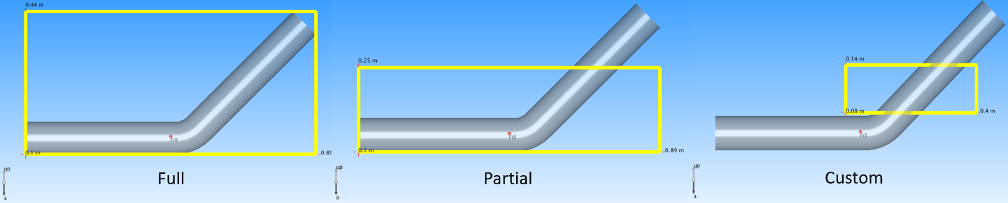
To illustrate the three Domain Mode options, consider the image below.

In the left-hand pane, the domain is set to Full. As such, the lattice represents a cubic bounding box containing all imported geometry.

In the center pane, the domain is set to Partial. Under this setting, the height of the box in the Up Direction can be adjusted, while the dimensions of the box perpendicular to the Up Direction are set to contain all imported geometry.

In the right-hand pane, the domain is set to Custom. In this configuration, the bounding box can be given an arbitrary location and extent.

Up Direction

For convenience with multi-fluid model building and setup, users can define a model “Up Direction.” The Up Direction typically points in the opposite direction of gravity, and provides ease-of-use functionality when defining partially filled tanks or initially stratified fluids. This reference dihedron can be seen on the viewing panel. By default, the Up Direction points in the +y direction, and gravity points in the -y direction. This default can be changed in the Edit > Preferences menu.

Fill Options

For a lattice domain that contains vessels, pipes, vials, tanks, etc., the solver needs to differentiate the interior zone of the lattice domain from the exterior zone. The interior zone is a continuous region within the lattice domain that, at some point during the simulation, may contain fluids, particles, species, or moving solid surfaces. These interior regions are typically the space inside a vessel, pipe, or bounding geometry. The exterior zone, which typically occupies the region between the outside tank walls and the lattice domain, will never contain fluid or particles.

To discriminate interior from exterior zones, the solver performs a 3D flood fill beginning at a user-defined fill point and then expands to the vessel walls and/or the simulation bounding box. By default, the fill point is set to the center of the main lattice domain. Users can move the flood fill point to other locations inside the domain or add multiple flood fill points, using the Edit Fill Point form on the context-specific toolbar.

To differentiate interior from exterior regions, the user must provide the location of an interior flood fill point. The solver then performs a 3D flood fill, expanding from this fill point to the walls of the body and/or the simulation bounding box. The region of the simulation domain that is touched by the flood fill is identified as an interior zone. The region that is not touched by the flood fill is identified as an exterior zone, and is excluded from the calculation.

Flood Fill

The location of the flood fill point.

Domain Center

The position of the flood fill location is the center of the lattice domain. The user can see the coordinates, but cannot adjust the coordinates.

Custom

The user enters a custom point as the flood fill seed location. The user can see the current coordinates and adjust the coordinates as needed.

Fluid Fill 1

m | The x-, y-, and z-coordinates of the flood fill seed location.

Note

• The flood fill point is shown in the 3D view. In most cases, the default flood fill location (Domain Center) is acceptable.

• In some cases however, such as U-tube manometers, toroidal geometries, or tanks with interior support structures, the point must be relocated to a location interior to the vessel.

• For all simulations, the interior volume calculated during the flood fill routine is reported to the simulation output log. If this calculated volume is in significant disagreement with the expected tank volume, check the flood fill point.

To illustrate the effect of flood fill seed location, consider the two flood fill results below. In image (A), the flood fill point was located inside the vessel in a region that is known to contain fluid during the simulation. Appropriately, the active region of the lattice domain is inside the tank, while the inactive region is outside the tank.

In image (B), the flood fill point was inappropriately located outside the vessel. The active region of the lattice domain is inappropriately located outside the tank, while the inactive region is inside the tank.

Further illustration is presented below, for a system involving flow around a bend. In image (A), the flood fill point is located inside the pipe. The flood fill algorithm expands to the sidewalls of the pipe and the lattice bounding box. The interior zone is (correctly) inside the pipe elbow. The exterior zone is (correctly) located outside the elbow. Regions in the active zone will be modeled. Those in the inactive zone will not be modeled.

In image (B), the flood fill point is located outside the pipe. The flood fill algorithm again expands to the sidewalls of the pipe and the lattice bounding box. The interior zone is incorrectly located outside the pipe. The flood fill point needs to be located inside the pipe on order to make the inside of the pipe the active zone.

A final illustration is presented below. In this example, we model species transport between two tanks connected by a small pipe. In image (B), improper selection of the point leads to improper active versus inactive zones.

Important

• The results of the flood fill algorithm are recorded in the BoundaryConditions.txt file, which can be rendered in M-Star Post under the Volume Fraction option. Regions where the reported fluid value is equal to 0 are inactive simulation zones which were untouched by the flood fill.

• Simulations predicting non-physical forces on moving objects (e.g., giganewtons) and/or zero fluid velocity despite the presence of a momentum source often result from an improper flood fill point location.

• If most of the simulation zone is inactive, consider using a sparse mesh to improve runtime speed and decrease memory requirements.

• Use culling zones for highly sparse lattices (where most cells do not contain fluid).

Dynamics

Linear and centripetal accelerations can also be imposed on the lattice. These accelerations can be constant or time-varying. By default, a constant acceleration of 9.81 m²/s is imposed on -y direction of the main lattice. Additional accelerations can be superimposed onto the system.

Gravity

m/s ² | The x-, y-, and z-components of the constant gravity vector.

External Accelerations

Applies an acceleration to the complete domain to mimic movement that is applied to the domain. It is easier to apply this acceleration than to model the motion directly. You can model a user-defined function to define your own custom motion. It is used for cell culture beds, shaken bottles, and microtiter plates. These points will be discussed in the forthcoming External Accelerations How-to Guide.

None

Object is at rest. No external acceleration.

Linear Shake

One-dimensional rigid body oscillation.

Orbital Shake

Two-dimensional rigid body orbital motion.

Rocking

One-dimensional rigid body rocking about a user-defined pivot point.

Ball Joint

Rigid body rotation on a ball joint.

Custom Rotation

Custom-defined rigid body rotation.

Custom Translation

Custom-defined rigid body translation.

System Boundary Conditions

The six sidewalls of the main lattice domain are, by default, assigned no-slip wall boundary conditions. In this condition, the lattice domain provides six rigid walls through which fluid, species, and/or particles cannot cross. The individual faces of the bounding box can be alternatively assigned velocity, pressure, and/or free-slip boundary conditions. For systems with openings, such as a pipes entering a tank, users can impose local boundary conditions along specific regions of the lattice domain. Multiple boundary conditions can be imposed on a single side of the lattice domain.

Local boundary conditions can be imposed at user-defined regions of the lattice domain. These local boundary conditions can be different from the lattice domain boundary condition. By default, the top surface (defined relative to the simulation Up Direction) is free slip, while the remaining five sides are no slip.

Min XBC

The minimum X plane boundary conditions.

No Slip

Zero fluid velocity along the bounding box wall​.

Free Slip

Zero fluid shear stress in the direction parallel to the wall; zero fluid velocity in the direction normal to the wall.​

Min YBC

The minimum Y plane boundary conditions.

No Slip

Zero fluid velocity along the bounding box wall​.

Free Slip

Zero fluid shear stress in the direction parallel to the wall; zero fluid velocity in the direction normal to the wall.​

Min ZBC

The minimum Z plane boundary conditions.

No Slip

Zero fluid velocity along the bounding box wall​.

Free Slip

Zero fluid shear stress in the direction parallel to the wall; zero fluid velocity in the direction normal to the wall.​

Max XBC

The maximum X plane boundary conditions.

No Slip

Zero fluid velocity along the bounding box wall​.

Free Slip

Zero fluid shear stress in the direction parallel to the wall; zero fluid velocity in the direction normal to the wall.​

Max YBC

The maximum Y plane boundary conditions.

No Slip

Zero fluid velocity along the bounding box wall​.

Free Slip

Zero fluid shear stress in the direction parallel to the wall; zero fluid velocity in the direction normal to the wall.​

Max ZBC

The maximum Z plane boundary conditions.

No Slip

Zero fluid velocity along the bounding box wall​.

Free Slip

Zero fluid shear stress in the direction parallel to the wall; zero fluid velocity in the direction normal to the wall.​

Note

For simulations involving closed tanks where the interior never touches the lattice domain side walls, the lattice domain boundary condition is of no consequence.

Display Attributes

Visible

The ability to show or hide the object.

Shown

The object is shown in the 3D view.

Hidden

The object is hidden in the 3D view.

Mode

This offers two options to view the object.

Wire

The object is shown as a wire frame.

Width

The width of the line used to render the object in the 3D view.

Shaded

The object is shown as a shaded surface.

Material

This allows the user to change the material of the object with the following options: Aluminum, Steel, Chrome, Plastic, or Glass.

Opacity

This scale allows the user to change the opacity of the object.

Color

This offers to change the color of the object.

Main Lattice Toolbar

Context-Specific Toolbar Forms	Description
Edit Box	The Edit Box form exposes handles along the six sides of the bounding box which can be dragged to stretch or move the geometry.
Edit Fill Points	The Edit Fill Points form defines the number and position of flood fill points in your system.
Reset box	The Reset Box command snaps the bounding box back to imported static geometry.
Volume Calculator	The Volume Calculator calculates the fluid volume.
Help	The Help command launches the M-Star reference documentation in your web browser.

For a full description of each option, see Context-Specific Toolbar selections.