Liquid Droplets

Introduction

Droplets are interacting Lagrangian spheres that move continuously through the fluid lattice. They are primarily used to model dispersed two-fluid systems, such as droplet suspensions, but are also effective for representing blending in density-stratified miscible fluids.

Each droplet consists of a rigid core that interacts elastically with other dispersed-phase particles. These hard-sphere interactions preserve incompressibility of the dispersed phase prior to breakup or dispersion. Surrounding the core is a fully penetrable concentric shell that increases the apparent particle volume. This “cherry-pit” construction allows the dispersed phase volume fraction to exceed the random packing limit (~0.64) of rigid spheres by accounting for interstitial space, enabling reconstructed volume fractions approaching 1.0, while still allowing the field to break up into smaller droplets.

Droplets are introduced as monodisperse particles within the Particle Injection of a droplet parent. During the simulation, droplets will typically undergo breakup into much smaller structures, with final sizes often orders of magnitude smaller than the initial diameter. Droplet volume fraction and size distribution can also inform local fluid rheology through user-defined models.

Droplet positions and velocities evolve according to Newton’s Second Law, using a Verlet integration scheme, with forces defined by the user. Each droplet is assigned a unique ID, birth timestamp, diameter, and origin ID upon entering the simulation. The birth timestamp enables computation of residence time distributions and mean age, while the origin ID tracks the source of each droplet. This allows analysis of mixing between streams and differentiation of droplets with varying properties (e.g., density or size) based on their origin.

Breakup and coalescence can be modeled at either the individual droplet level or using a parcel-based approach. In both cases, the resulting droplet size distribution is governed by fluid kinematics and droplet material properties. Individual-level models resolve pairwise interactions, while parcel approaches capture ensemble behavior more efficiently.

Mass transfer between droplets and the surrounding fluid is supported through user-defined correlations. The mass transfer rate for each droplet is computed from a local mass transfer coefficient and the concentration difference between the droplet and fluid phases. Resulting mass exchange leads to droplet growth or shrinkage while conserving total species mass.

Adding Liquid Droplets

When adding particles to a system, there are two factors to consider: (1) the number of particles entering the system, and (2) the location of the particles entering the system.

1. The number of particles entering the system is defined by an injection rate and an injection duration. Pay close attention to the appropriate number of particles added to the system as very large particle counts can slow performance. Various injection options are provided for defining these parameters.

2. The location of the particle injection is typically defined using an injection zone, an inlet boundary condition, or a background injection:

   • A particle injection allows users to define custom injection regions with local injection rates, injection size distributions, and initial particle compositions that differ from those defined on the particle parent. Particle injections allow for differentiated particle characteristics within a particle family. Children geometry can be added to the injection to control where particles are added to the system.

   • An inlet boundary condition represents the superposition of particles on the fluid field along the boundary condition surface. Boundary condition flow sweeps these particles from the initial positions along the boundary condition to other regions in the system.

   • A background injection produces a uniform distribution of particles across the full fluid field. This addition, if applied at the start of a process, represents a system with an initially well-dispersed ensemble of particles.

Liquid Droplets can also enter the system through Eularian conversion and volumetric generation via a user-defined function. Eularian conversion is used to model fluid-to-fluid conversion processes, as realized during jet breakup, air entrainment, and two-fluid dispersion processes. Volumetric generation is used to model particle nucleation, particle crystallization, and so forth.

Note

Use caution when adding more than a billion particles. System memory limits the total number of particles that can be tracked. On a single workstation, this limit is 50–100 million particles. On a GPU cluster, this limit is about 1 billion particles.

Property Grid

General

Density

kg/m ³ | Density of the dispersed phase droplets.

Note

In addition to hard sphere droplet-droplet interactions, the trajectories of each droplet are informed by the weight, buoyancy, drag, and virtual mass forces.

Forces and Fluid Coupling

Liquid droplet particles are modeled as Lagrangian objects that move according to Newton’s second law. Within this framework, the time-evolution of the particle acceleration vector is linked to the sum of the external forces acting on the particle via the particle mass. The particle mass is calculated automatically from the instantaneous particle density and diameter.

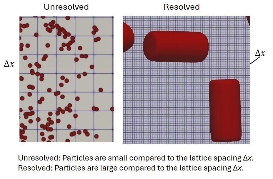
Both unresolved and resolved liquid droplet representations are available. Most simulations use an unresolved particle representation. Unresolved particles are small compared to the lattice spacing, and the flow field around the particle is not explicitly resolved. As such, for unresolved particles, interactions (e.g., particle drag, lift) are modeled using empirical correlations. These interactions can be either one-way or two-way coupled to the fluid.

Resolved particles are large compared to the lattice spacing, meaning the flow field/boundary layer around the particle is resolved explicitly. Resolved models do not evoke any user-defined drag or lift coefficient; rather, since the flow is resolved, these forces are computed directly from the fluid field surrounding the particle. The fluid/particle forces are automatically two-way coupled. Resolved simulations are an advanced modeling technique which typically require a large simulation resolution.

For both representations, custom forces and/or additional external forces can be defined via a UDF. For more discussion of these fluid particle forces, see the additional forces and fluid coupling overview.

Representation

This option specifies how the particles will be represented in the system.

Unresolved

Particles are assumed to be small compared to the lattice spacing. Fluid forces are calculated from user-set drag/lift relationships.

Resolved

Particles are assumed to be large compared to the grid spacing. Fluid forces are calculated directly from the flow field.

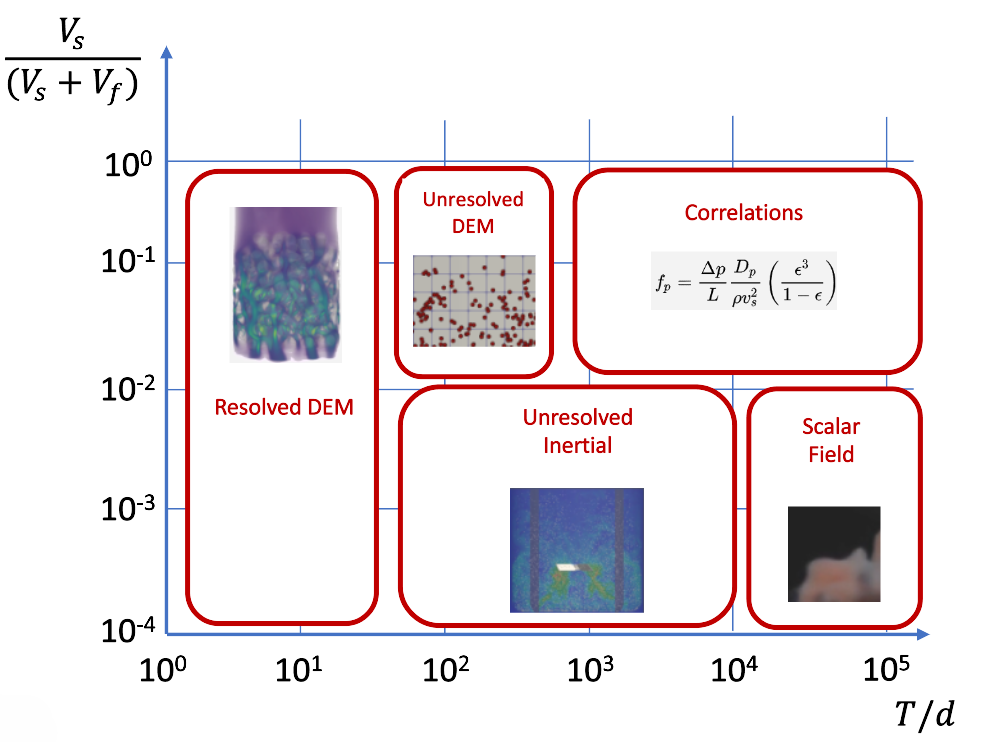
The following graph indicates when to use resolved versus unresolved particles.

If a static body is present, the following section will launch:

Static Body Interaction

This parameter specifies how each particle set interacts with each solid body family. When bounce interactions are specified, the contact force is calculated using a Hertz contact model. Pass through and stick boundary conditions can also be specified.

Static Body Option

This parameter specifies how each particle set interacts with each solid body family.

Bounce Simple

Particle-solid interactions are calculated using the Hertz contact model. The properties of the solid wall, as used to calculate overlap and stiffness, are assumed to be:

Static Body Poisson Ratio

0.3

Static Body Young’s Modulus

GPa | 0.1

Static Body Wall Coefficient of Restitution

0.1

Static Body Wall Sliding Friction Coefficient

0.5

Bounce Custom

Particle-solid interactions are calculated using the Hertz contact model. The properties of the solid wall, as used to calculate overlap and stiffness, are defined by the user. Default values are the properties evoked when using the Bounce Simple interaction option.

Static Body Poisson Ratio

0.3

Static Body Young’s Modulus

GPa | 0.1

Static Body Wall Coefficient of Restitution

0.1

Static Body Wall Sliding Friction Coefficient

0.5

Stick

The particles stick to the solid surface. No physical properties are specified, and the particles remain stuck to the surface through the simulation. The motion control option, combined with an appropriate set of custom particle variations, should be used if more sophisticated stick and/or stick/release conditions are required.

Pass Thru

The particles do not interact directly with the solid body family.

If a moving body is present, the following section will launch:

Moving Body Interaction

This parameter specifies how each particle set interacts with each moving body family. When bounce interactions are specified, the contact force is calculated using a Hertz contact model. Pass through and stick boundary conditions can also be specified.

Moving Body Option

This parameter specifies how each particle set interacts with each moving body family.

Bounce Simple

Particle-solid interactions are calculated using the Hertz contact model. The properties of the moving wall, as used to calculate overlap and stiffness, are assumed to be:

Moving Body Poisson Ratio

0.3

Moving Body Young’s Modulus

GPa | 0.1

Moving Body Wall Coefficient of Restitution

0.1

Moving Body Wall Sliding Friction Coefficient

0.5

Bounce Custom

Particle-solid interactions are calculated using the Hertz contact model. The properties of the moving wall, as used to calculate overlap and stiffness, are defined by the user. Default values are the properties evoked when using the Bounce Simple interaction option.

Moving Body Poisson Ratio

0.3

Moving Body Young’s Modulus

GPa | 0.1

Moving Body Wall Coefficient of Restitution

0.1

Moving Body Wall Sliding Friction Coefficient

0.5

Pass Thru

The particles do not interact directly with the moving body family.

Breakup/Coalesce

Particle breakup and coalescence can be modeled using either discrete or parcel-based representations.

In the discrete representation, particle breakup occurs on a particle-by-particle basis and generates a new particle that is explicitly tracked in the simulation; this new particle inherits the properties of the mother particle from which it was broken off. Particle coalescence is regulated at the level of individual particle pairs by comparing the approach Reynold’s number to a critical coalescence parameter. Coalescence events reduce the number of explicitly tracked bubbles.

In the parcel-based representation, both particle breakup and coalescence are regulated implicitly by adjusting the number scale associated with each parcel. Changes in diameter are informed by the local fluid properties which, when combined with surface tension and density, define an equilibrium particle diameter. With this approach, the number of explicitly tracked particles does not change due to breakup or coalescence events. See additional breakup/coalesce overview.

Breakup Enabled

Particle breakup typically occurs on the level of individual particles and is informed by the physical properties of the particle and the kinematic properties of the fluid.

Coalesce Enabled

Coalescence typically occurs at the level of particle pairs and is informed by the kinematic properties of the two particles.

Interfacial Mass Transfer

Interfacial mass transfer is calculated on a particle-by-particle basis using the local and instantaneous fluid and particle properties. This can be represented as either a convective transfer coefficient, \(k_L\), or a particle dissolution rate. In principle, the convective transfer coefficient and the dissolution rate describe very similar physical transport processes. In practice, a convective transfer coefficient is typically applied to gas bubbles and a dissolution rate is applied to solid particles.

Download Sample File: Scalar Coupling

Mechanically speaking, the convective transfer coefficient describes the rate at which mass is transferred (via convection) through the fluid boundary layer surrounding the particle. This rate is often written in terms of the local fluid energy dissipation rate, fluid viscosity, and fluid diffusion coefficient; although, in many cases a constant transfer coefficient may be suitable.

Theoretically speaking, most convective mass transfer models are developed under the assumption that the fluid immediately surrounding the particle remains fully saturated throughout the transport process. The rate at which mass is transferred into the system is therefore a function of the rate at which the saturated fluid adjacent to the bubble surface can be engulfed into the fluid bulk. These transfer functions can be derived from semi-empirical boundary layer theory.

Conversely, particle dissolution rates are developed under the assumption that the dissolved species concentration is low relative to the solid phase concentration. As such, the transfer rate is often related to the system temperature and the physiochemical properties of the solid rather than to the convective properties of the fluid surrounding the solid. In many cases, the dissolution rate is set to a constant value determined empirically.

Framework

This parameter determines whether mass transfer is modeled using the convective transfer coefficient or the particle dissolution rate. These values are calculated on a particle-by-particle basis using the local and instantaneous particle and/or fluid properties.

Convection

This calculates a convective mass transfer coefficient for each particle. Input to this expression includes the local and instantaneous properties of the particle and surrounding fluid.

kL UDF

m/s | This UDF defines the convective mass transfer coefficient in the fluid surrounding a particle. One output must be defined within the UDF: a floating-point variable named kl_{Particles}, where {Particles} is the dynamic name of the particle set. This output value is used when predicting convective mass transfer processes, including mass exchange with coupled scalar fields. This is a particle-based local UDF, calculated on a particle-by-particle basis using the local particle/fluid properties.

Download Sample File: kL

Dissolution

This calculates a dissolution rate for each particle. Possible input to this expression includes the local and instantaneous properties of the particle and surrounding fluid.

Dissolution Rate UDF

\(\frac{kg}{m^2 \cdot s}\) | This UDF defines the particle dissolution rate, defined here as the rate at which mass is exchanged between the solid phase (particles) and the dissolved phase/solute (coupled scalar field). One output must be defined as within the UDF: a floating point variable named dr_{Particle Set Name}, where {Particle Set Name} is the dynamic name of the particle set parent.

This output value defines the particle-specific dissolution rate. Positive values imply dissolution (mass leaving the particle). Negative values imply precipitation or crystallization. The units on the output variable are kg/m ² /s. This is a particle-based local UDF, calculated on a particle-by-particle basis using the local particle/fluid properties.

Download Sample File: Dissolution Rate

None

No mass transfer coefficient or dissolution rate is calculated.

If Interfacial Mass Transfer is on and a scalar is added, the following section will launch:

Scalar Coupling

Coupling Method

This option determines if particle-fluid scalar coupling is active in the simulation and whether it is modeled using built-in or user-defined functions. See additional scalar coupling overview.

Automatic

Predefined convection and/or dissolution models determine scalar transport rate, calculated on a particle-by-particle basis. The units on these properties depend on system setup and must be dimensionally homogeneous. Transport by convection is calculated from the user-specified convective transfer coefficient, the particle surface area, and the differences between the local concentration and the saturation limit. Transport by dissolution is calculated using the dissolution rate and the particle surface area. The same transport model is applied to all species participating in interfacial mass transfer.

Custom

User-defined transport models determine scalar transport rate, calculated on a particle-by-particle basis. These models could include the user-defined convective transfer coefficient, the user-defined dissolution rate, particle custom variables, or arbitrary functions of the local fluid/properties. A unique transport model can be specified for each species. The user must confirm that the transport parameters are dimensionally homogeneous.

None

No particle-fluid scalar coupling is considered. Although a convective transfer coefficient or dissolution rate may be defined, no species will be transferred between the particles and fluid.

If a Thermal Field is added, the following section will launch:

Thermal Coupling

The thermal coupling option enables users to model time-dependent particle temperature evolution. Temperature changes may arise from either intra-particle reactions or heat exchange between particles and the surrounding fluid. Intra-particle heat generation or consumption is computed on a particle-by-particle basis, allowing each particle to evolve independently according to its local reaction kinetics.

Heat exchange between a particle and the fluid is likewise evaluated individually for each particle, using the local fluid properties in the surrounding computational voxels. These particle–fluid heat transfer processes are two-way coupled. The heat flux between phases appears as a source or sink term in the fluid energy equation while simultaneously modifying the particle temperature.

Track Temperature

This option determines if particle temperature is tracked during the simulation. Temperature changes can be caused by endo- or exothermic intra-particle reactions or heat exchange with the surrounding fluid.

Off

Particle temperature is not tracked during the simulation.

On

Particle temperature is tracked during the simulation.

Initial Temperature

K | This parameter defines the initial temperature of the particles in the set.

Heat Capacity

J/m ³ K | This parameter defines the heat capacity of the particles. The heat capacity informs how changes in the thermal energy affect changes in temperature.

Fluid Particle Heat Transfer Coupling Method

The coupling method determines if particle-fluid scalar coupling is active in the simulation and whether it is modeled using built-in or user-defined functions.

None

No particle–fluid heat transfer is considered. The particle temperature changes only due to endothermic or exothermic intra-particle reactions.

Convection

When using Convection, the species mass transfer rate between a particle and the surrounding fluid is informed by the heat transfer coefficient, the particle surface area, and the local temperature difference between the particle and the fluid,

\[\dot{q}_{T_p} = h_p A_p (T_p - T_f)\]

where \(\dot{q}_{T}\) is the heat transfer rate between particle \(p\) and the surrounding fluid, \(h_p\) is the convective transfer coefficient of the fluid surrounding the particle, \(A_p\) is the area of particle, \(T_p\) is the temperature of the particle, and \(T_f\) is the temperature of the fluid surrounding the particle.

Within this framework, the heat transfer coefficient of each particle \(h_p\) is calculated using the model of Deckwer, which combines Higbie’s penetration theory with Kolmogoroff’s theory of isotropic turbulence,

\[h_p = 0.1 C_v (\varepsilon \nu)^{1/4} \left( \frac{\alpha}{\nu} \right)^{1/2}\]

where \(C_v\), \(\nu\), and \(\alpha\) are the specific heat (at constant volume), kinematic viscosity, and thermal diffusivity of the fluid.

UDF

The user defines a custom fluid-particle heat transfer rate.

Heat Transfer UDF

W | This UDF defines the heat transfer between particles and the surrounding fluid. One output must be defined within the UDF: a floating-point variable named Qdot. This output variable defines heat flow between the particle and the surrounding fluid. Positive values imply heat transfer into the particle (from the surrounding fluid). Negative values imply heat transfer away from the particle (into the surrounding fluid). The functional form of the heat transfer model is discussed in the particle heat transfer overview. This is a particle-based local UDF, calculated on a particle-by-particle basis using the local particle/fluid properties.

Download Sample File: Heat Flux

Advanced

DEM Bounce Method

This options for this method defines how the particles interact with solid bodies. The example below shows the difference between the two options.

Voxel

This is the default option. It is computationally faster than the Triangle method. The particles interact with the boundaries of the fluid voxels. Smaller particles can get caught on the “steps” for coarser resolutions. As the lattice resolution increases, this effect is minimized.

Triangle

In this option, the particles interact with the triangles made from the tessellations of the static body surface. This is more computationally expensive than the Voxel option, but results in a more physically realistic interaction with the static body. The size of the triangles used to represent the surface are set using the edit mesh form. The corresponding mesh can be previewed using the Preview Surface Meshes tool.

Signed Distance

Particles that penetrate the wall are moved back into the system based on the signed distance field they moved into the wall. This correction is numerical and not linked to the physical properties of the particles.

Compute Nearest Neighbor Distribution

Computes the average nearest neighbor separation distance and nearest neighbor separation distance probability distribution function. See additional discussion in Theory: Nearest Neighbor Distribution. The Particle Output Data page describes the output for this option.

On

Particle distribution data are computed.

Off

Particle distribution data are not computed.

Enable Movement Control

With this option, users can define a UDF that conditionally controls whether particles are moving or fixed. Particle motion can be reactivated as part of the UDF.

On

Movement control of particles is enabled. Individual particles may become fixed in space per some user-defined condition.

Movement Control UDF

none | This UDF defines if individual particles move or remain fixed in space. One of two possible boolean outputs can be defined as part of the UDF: makeFixed and makeMoving. The values assigned to each value can change over time. If the boolean makeMoving is set to true, the particle will evolve through space. Only one boolean should be true at each time step. This is a local UDF, calculated on a particle-by-particle basis using the local particle/fluid properties.

Download Sample File: Movement Contol

Off

No controlled movement of particles. Particles always have the ability to move through space.

Compute Pressure Gradient Force

When this option is active, the pressure gradient force on the particle is calculated. This force acts from regions of higher pressure toward regions of lower pressure, influencing the motion of particles immersed in the fluid.

For a small particle within a fluid, the pressure gradient force can be expressed as:​

\[F_p = - V_p \nabla P\]

where \(V_p\) is the volume of the particle and \(\nabla P\) is the pressure gradient and the location of the particle.

Off

Does not compute pressure gradient force.

On

Computes pressure gradient force.

Enable Removal UDF

Enable removal user-defined function.

Removal UDF

no units | This UDF removes particles based on particle properties or local fluid conditions. One output must defined within the UDF: a Boolean variable named remove. This output value determines if a particle is to be removed from the simulation. If set to true, the particle is removed. This is a local UDF, calculated on a particle-by-particle basis using the local particle/fluid properties.

Download Sample File: Removal

Enable Particle Density UDF

TBA

Off

Particle Density UDF not enabled.

On

Particle Density UDF enabled.

Particle Density UDF

TBA

Download Sample File: Particle Density

Liquid Droplets Output Data

Particle output data is summarized on the Particle Output Data page. These outputs include individual particle motion and properties, ensemble statistics, spatial fields constructed from the local particle population, as well as particle exit statistics.

Liquid Droplets Toolbar

Context-Specific Toolbar Forms	Description
Add Particle Injection	The Add Particle Injection adds an injection to a particle parent.
Add Particle Scalar	The Add Particle Scalar tool assigns custom properties to individual particles which move with them and can be used to model intraparticle reactions.
Add Particle Reaction	The Add Particle Reaction tool applies user-defined kinetics to each particle based on its composition and surrounding fluid properties.
Add Particle Variable	The Add Particle Variable tool defines per-particle quantities via UDFs, accessing particle properties and local fluid conditions.
Diagnostics	The Diagnostics form reports the position, orientation, and moments of inertia associated with a static body.
Help	The Help command launches the M-Star reference documentation in your web browser.

See also Child Geometry Context Specific Toolbar.

For a full description of each selection on the Context-Specific Toolbar, see Toolbar Selections.

Additional Resources

For more on this subject, check out the following:

Publications

• Predicting the diameters of droplets produced in turbulent liquid–liquid dispersion