Particle Reaction

Introduction

Particle body reactions represent chemical reactions that operate inside particles. The reactions are calculated on a particle-by-particle basis and can be a function of the particle properties, particle scalar values, particle custom variables, local fluid properties, as well as any global variables or parameters.

Particle reactions can also interact with aqueous scalar fields, provided the scalar field is coupled to the particles via a convection or dissolution/perception process. When a thermal field is active, particle reactions can include the effects of heat of reaction (i.e., exothermic and endothermic reactions).

Particle reactions are useful for modeling particle curing processes, intracellular reactions, particle polymerization processes, etc.

Mathematically speaking, particle reactions are ordinary differential equations that describe how species concentrations and other values within each particle change as a function of time. These reaction kinetics are written as species-specific rate equations, which are typically linked to a chemical equation using the law of mass action and an associated reaction rate. This point is discussed in the example above.

Particle reactions are typically solved explicitly using either a 1st order Euler or a 4th order Runge-Kutta solver. The solution step size in both approaches is set to the simulation time step. An implicit solver based on the Rosenbrock method is also available for systems with fast reaction kinetics (e.g., stiff equations).

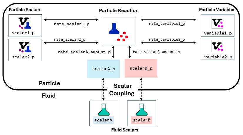
Within the Particle Reaction UDF, as illustrated in the figure below, reaction rates can be specified for all particle scalars and particle variables associated with the particle set. These reaction rates describe how the species concentration changes over time in response to local fluid/particle properties. Reaction rates can also be specified for any coupled scalar field, although these operate on the amount of coupled scalar contained within the particles (as opposed to the concentration.) If a thermal field is present, a heat of reaction can be also specified. A positive heat of reaction will heat the particles. A negative heat of reaction will cool the particles.

The rates defined in the particle reactions can be a function of particle scalars, particle variables, local species concentrations, or any of the typical fluid variables (e.g., strain rate, energy dissipation rate, temperature). All particle scalars and variables associated with the particle family can be updated in the same particle reaction UDF; separate particle reactions are not needed for each scalar.

Property Grid

Intraparticle Reaction UDF

mol/s, g/s, or none | This UDF defines intraparticle reactions between species inside a particle. The number of output variables matches the total number of coupled aqueous and particle scalar fields in the model. The output variables are named rate_{scalar}, where {scalar} is the dynamic name of the coupled scalar field, and rate_{pvs_p}, where {pvs_p} is the dynamic name of the particle species. Each output is a floating-point value representing the reaction rate.

Rates can be specified for all particle scalars, as well as species coupled to the scalar field. The interspecies reaction rate must have units compatible with those defined for the interparticle species concentration. Positive values indicate species production, while negative values indicate species consumption.

If a thermal field is present and the heat of reaction is enabled, an additional QDot output becomes available. Positive QDot values imply exothermic reactions, whereas negative values indicate endothermic reactions.

This is a particle-based local UDF, calculated on a particle-by-particle basis using the local particle/fluid properties.

In the example below, we model a curing process wherein resin particles are converted into product particles. The curing process is driven by a miscible solvent, which is added to the top of the vessel. The curing process requires a minimum local solvent concentration to initiate particle conversion. Above a certain solvent threshold, the resin converts into an undesired byproduct. The competition between solvent mixing and particle-solvent exposure informs the batch processing time and the final process selectivity.

The animation on the left illustrates solvent mixing and particle suspension due to ongoing agitation. The solvent blend time is approximately 30 seconds. The histograms on the right illustrate distributions of (i) particle yield and (ii) the amount of resin remaining on the particles. The particle yield, shown as the top histogram, describes the ratio of desired product to total product. A selectivity of 1 implies that all resin was converted into the desired product. A selectivity of 0 implies that all resin was converted into a byproduct. In this example, the final selectivity after 30 seconds of agitation varies between 0.2 and 1.0.

The bottom histogram presents the distribution of resin remaining on the particles. When first added to the system, all particles have 1 mol of resin. As the particles react with solvent and cure, the amount of resin remaining on each particle decreases from 1 mol to zero. Owing to local variations in the solvent concentration, some particles cure faster than others. This behavior leads to time-evolving variation in the distribution function. After approximately 30 seconds, all particles are fully cured.

Download Sample File: Particle Reaction

Integration

This setting defines which algorithm will be used to numerically integrate the reaction kinetics.

Euler (1st Order)

A first-order forward Euler method advances species concentration. For species \(A\) with concentration \([A]\), this becomes:

\[[A]_{t + \Delta t} = [A]_t + \frac{d[A]}{dt} \Delta t\]

Where \(\frac{d[A]}{dt}\) is the reaction rate defined in the Reaction UDF and \(\Delta t\) is the simulation time step.

Runge-Kutta (4th Order)

A fourth-order Runge-Kutta method advances species concentration. For species \(A\) with concentration \([A]\), this becomes:

\[[A]_{t + \Delta t} = [A]_t + \frac{\Delta t}{6} \left(k_1 + 2k_2 + 2k_3 + k_4\right)\]

where

\[ \begin{align}\begin{aligned}k_1 = f(t, [A]_t)\\k_2 = f \left( t + \frac{\Delta t}{2}, [A]_t + \frac{\Delta t}{2} \, k_1 \right)\\k_3 = f \left( t + \frac{\Delta t}{2}, [A]_t + \frac{\Delta t}{2} \, k_2 \right)\\k_4 = f \left( t + \Delta t, [A]_t + \Delta t \, k_3 \right)\end{aligned}\end{align} \]

with

\[f(t, [A]_t) = \frac{d[A]}{dt}\]

Rosenbrock (Implicit)

An implicit Rosenbrock method advances species concentrations. This approach is recommended for systems with fast reactions that introduce numerically stiff kinetics. Although more computationally expensive than explicit methods, Rosenbrock is preferred when explicit stability criteria require time steps smaller than those needed to resolve the flow’s behavior.

Rosenbrock methods are a subclass of linearly implicit Runge-Kutta schemes. They linearize the implicit system at each time step, requiring only the solution of linear systems rather than nonlinear ones. The solver evaluates stage derivatives using the Jacobian of the reaction source term without iterative solvers. This structure allows Rosenbrock methods to efficiently integrate stiff chemical kinetics while maintaining second- or higher-order accuracy.

The implementation follows the framework of Sandu et al.

Particle Reaction Toolbar

Context-Specific Toolbar Forms	Description
Help	The Help command launches the M-Star reference documentation in your web browser.

For a full description of each option, see Context-Specific Toolbar selections.