V-Blender DEM Model

This is a guide to take you step by step to build a DEM model for mix two different compounds modelled as DEM particles. As well, we will learn how to measure the mixing index and implement it as part of the simulation output.

The problem

Original Statement:

We want to mix two different powder components and asses the mixing efficiency/homogeneity after a pre-stablished time (or number of rotations).

The mixer is a V-shape vessel with a horizontal intensifier bar across its middle section. The intensifier bar is composed of a horizontal bar with 2 welded discs tilted 10°, those discs have 4 arms joint on their perimeter.

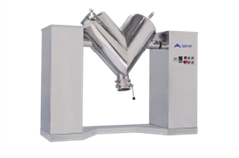
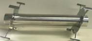
V-shape mixer and intensifier bar detail.

The different compounds are introduced separately in the vessel from each one of upper inlets. The powder compounds would be released in sequence, creating two layers in the vessel with the higher mass powder at the bottom and the lower mass compound stacked on top.

Once the vessel is fill with the two powder compounds, and they are settled in the vessel, the mixing will start. The mixing motion can be divided in two different movements:

• Tumbling: the vessel rotates around its horizontal axis at 25 rpm.

• Intensifier rotation: the intensifier bar rotates around the same rotation axis as the V-shaped vessel at 1500rpm.

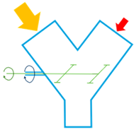
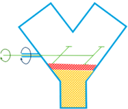
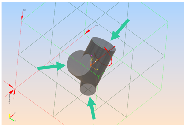
Diagram illustrating the mixer lay out, the filling process and the motion (rotation axis)

The mixing will run for 10 tumbling rotations and once the simulation is finish, we will assess the mixing index.

The compound properties used for this example are detailed below:

Particle properties

Particle properties	Rodent Feed 1	AI Feed 2	Units
Density of solid	500	688	kg/m3
Mass of solid	1.8	0.063	kg
Particle size (radius perfect sphere)	0.000097	0.000085	m

Problem definition:

Now, we need to plan how we are going to approach the proposed problem. For this we need to understand how the system works, what we want to achieve and the potential limitations that we could face.

It is clear we are facing a single phase fluid with DEM particles, due to the nature of the problem we will model the powder as DEM particles immersed in a single fluid (air).

The overall mixing process is clear, but let’s break it down chronologically:

• t=0, the Rodent Feed 1 is dumped into the V-shape vessel.

• t=2.5 seconds, the AI Feed 2 is introduced into the vessel.

• t=5 seconds, the V-shaped mixer movement starts with a linear ramp up (both the tumbling and intensifier rotation).

• t=7 seconds, the tumbling reaches max speed (25 rpm).

• t=15 seconds, the intensifier reaches max speed (1500 rpm).

• t=29 seconds, both, the tumbling and the intensifier start the ramp down of their movement.

• t=31 seconds, the system stops completely (tumbling and intensifier rotation).

• t=32 seconds, the simulation finish.

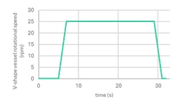
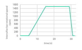
Rotational velocity profiles for V-shape vessel (tumble) and intensifier bar

Let’s explain some of the points listed above:

• The overall fill time for both powders has been set as 2.5 seconds to allow the components to settle and reach an equilibrium state.

• The vessel and intensifier bar rotation has been ramped up to working speed (and then rumped down to zero) to achieve a realistic mixing behaviour.

• The overall tumbling time (considering the ramping up and down) has been calculated to achieve 10 vessel rotations and ensure the system finish in vertical position. Taking 25 rpm, we know that every 12 seconds the system rotate 5 times; hence to achieve 10 rotations we require 24 seconds. However, as the vessel accelerates from 0 to max speed for 2 seconds and decelerates from max speed to 0 in another 2 seconds, we require two extra seconds to compensate. Overall, we have a tumbling time of 26 seconds.

• Once the tumbling finish, we leave the simulation running for an extra minute to allow the particles to settle.

Once we have a clear idea of what we are going to simulate, we must think on how we would run the simulation and what kind of limitations we can face. The main issue that we can identify from the data provided is the number of particles: based on the Rodent Feed 1 mass and particle size provided, we are looking at a simulation with over 11 billion particles with a very small size. This in one hand requires an enormous amount of ram to store the data and it will take days as the particles diameter will drive the whole resolution.

The proposal here is simple: develop a size sensitivity study to identify the biggest diameter that can deliver realistic results (the same mixing index) with a reduced computational cost. It is known that from a critical particle size, the mixing properties do not change. In another words: there is a value for the particle size below which the mixing behaviour is independent of the particle size. Identify this value is critical, as it will allow us to use larger particle sizes and obtain the same results than using the very fine ones. However, this particle size depends on each problem configuration (the mixer, the amount of each compound, etc) so we must do a sensitivity study for each case.

Below, we can see an example of the mixing index variation with the particle diameter, as it can be seen from ~0.5mm the mixing index stays the same. Which means that even if our particles are smaller than that (for example, the requirement is a diameter of 100 microns), we don’t need to model our DEM particles at that level because the mixing became independent of the particle size from 500 microns onwards.

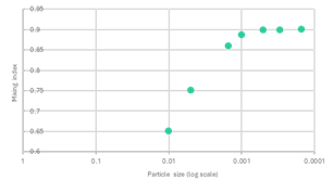
Mixing index vs. Particle size (diameter)

Just to be clear, we must develop a particle size sensitivity study, for doing this it is recommended start with large particles and reduce the size iteratively until we observe no change (or minimal) in the mixing index.

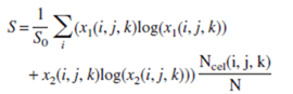
The last point that we must cover is how to assess the mixing efficiency/homogeneity. For this we will use a mixing index based on the entropy of the mixing, defined as:

\[S = \frac{1}{S_0} \sum_{i} (x_1(i,j,k)\log(x_1(i,j,k)) + x_2(i,j,k)\log(x_2(i,j,k))) \frac{N_{cel}(i,j,k)}{N}\]

Where: \(S_0\) is the entropy of a completely mixed system, which depends on the fraction of coloured particles in the system; \(x_1(i,j,k)\), \(x_2(i,j,k)\) are the fractions of the coloured particles in cell i, j, k; \(N_{cel}(i,j,k)\) is the number of particles in cell (i, j, k), N is the total number of particles in the system.

Let’s understand the above parameters:

• \(x_1\) and \(x_2\) represent the percentage of each particle on each single cell, this means we need to calculate the total number of particles in the volume, identify the number of particles in each cell and divide those values.

• \(N_{cel}\) is the total number of particles on each cell (species 1 and species 2 together).

• \(N\) is the total amount of particles (species 1 and 2) in the whole control volume.

With a clear idea of what we must do, we can proceed to build up the model.

Build the model

Geometry set up

From a geometrical point of view, the V-shape mixer is build based on two bodies: the V-shape vessel and the intensifier bar. Due to its complexity, it is assumed that those elements are provided (or created in a separate CAD software).

Both components would be rotating around the same axis, this makes things easier as we can set both up as moving bodies. If the rotation axis were different and one of the components is inside the other, then a different approach should be taken (ask M-Star support for further details).

1. Open M-Star Pre.

2. Import the CAD data in M-Star: as we know the bodies we are going to import in M-Star are moving elements we start by creating a moving body branch in the Model Tree:

   Create -> Moving Body -> Import from File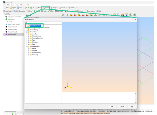

   

   Create Moving Body

3. A new window will open, navigate and select the file for the V-blender vessel, click open. It will load in the preview window -> hit OK to confirm. The V-shape vessel will appear in the window.

Now, we are going to consider a couple of good practices for any simulation:

• Name properly all the different components in the model: this will allow us to keep models tidy and well organized, making things easier for future uses, modifications and post processing.

• Always check the geometry: look around the geometry we have been provided, make sure it is the correct data, a good quality representation of the problem, that all the important components for the simulation are present, etc.

Applying the above recommendations:

• Rename the Moving Body as VShapedVessel.

• Pan around the CAD data: you can notice that the three edges of the vessel are open -> We must close them to ensure a watertight volume inside the mixer where we want to run our simulation.

Open surfaces for the V-shaped vessel.

Closing the vessel apertures is very easy, we will use the parametric geometry provided by M-Star Pre.

Right click on VShapedVessel -> Add Geometry -> Primitive -> Cylinder -> OK

A new part appears on the screen, and it will be added as a child geometry under the moving body we called VShapedVessel. Position the new cylinder using “Mate” and adjust the size to match the vessel inlet (radius 0.127m). Define the length as 1 mm, so it would be just a small cap to enclose the internal volume. Rename the geometry as CAP_LHS, CAP_RHS or CAP_Bottom as corresponding. Repeat this for the remaining two apertures (for the bottom cap, you can interactively measure the radius using the tool Measure Point to Point available in M-Star Pre).

Once the vessel is a closed volume, we can set up the motion characteristic. Select VShapedVessel (the moving body) and we can see the information related with this tree branch. The first thing we can see is the motion axis definition; we must define the correct motion axis -> Click Define axis -> The information window changes.

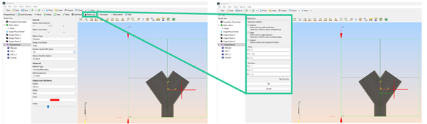
Motion axis definition

Input the point (axis location) and direction of the motion axis. As example, the motion axis is horizontal (1, 0, 0) and located at (0, -0.2, 0). Adjust as required. Click OK to accept.

Next, we must define the motion. Selecting again VShapedVessel (the moving body), on the information window (see below) we will introduce the following adjustments to match our problem requirements.

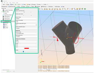
Moving body information window

• Motion Type -> Rotation

• Ramp Time Mode -> Off (if activated, the ramp up will start from t=0 and we can’t control the ramp down; this is not compatible with our problem approach with a delay start of the rotation, controlled ramp times and need of a ramp down -> we disable this option and define the rotational speed variations via UDF)

• Rotation Speed UDF (rpm) -> Open the editor and type:

  float omega = 25;
  float tstart = 5;
  float rampuptime = 2;
  float tumbletime = 22;
  float rampdowntime = 2;
  float tend = 31;
  
  if (t<tstart){
      value = 0;
  }
  if (t>tstart){
      if (t<tstart + rampuptime){
          value = (omega/rampuptime)*(t-tstart);
      }else{
          if (t<tstart + rampuptime + tumbletime){
              value = omega;
          }else{
              if (t<tend){
                  value = (omega/rampdowntime)*(tend-t);
              }else{
                  value = 0;
              }
          }
      }
  }
  

  This script replicates the rotational speed profile for the V-shaped vessel explained in the section Problem Definition -> Overall mixing process. If this profile is defined in a different way, the script must be modified accordingly.

• Motion Modifier option -> Disabled (we are interested in rotation only).

The Advanced options remain as they are.

Repeat this complete process for the Intensifier Bar, keep in mind the following things:

• The rotation axis must be the same as the one defined for the V-shaped vessel.

• Rotation Speed UDF (rpm) -> Open the editor and type:

  float omega = 1500;
  float tstart = 5;
  float rampuptime = 10;
  float tumbletime = 14;
  float rampdowntime = 2;
  float tend = 31;
  
  if (t<tstart){
      value = 0;
  }
  if (t>tstart){
      if (t<tstart + rampuptime){
          value = (omega/rampuptime)*(t-tstart);
      }else{
          if (t<tstart + rampuptime + tumbletime){
              value = omega;
          }else{
              if (t<tend){
                  value = (omega/rampdowntime)*(tend-t);
              }else{
                  value = 0;
              }
          }
      }
  }
  

  As before, this script will replicate the rotational speed profile for the intensifier bar explained in the section Problem Definition -> Overall mixing process. If this profile is defined in a different way, the script must be modified accordingly.

Fluid and domain set up

With all the geometry ready, including the motion, it is time to have a look at what would be the fluid in our simulation and how we define the fluid domain that we are interested.

As mentioned earlier, this simulation is clearly a single-phase model, this setting is default when starting a model from scratch. However, it is recommended to check it, if the modelling isn’t set to Single Phase Fluid, you can change the fluid configuration using the Fluid option in the top menu area in M-Star Pre.

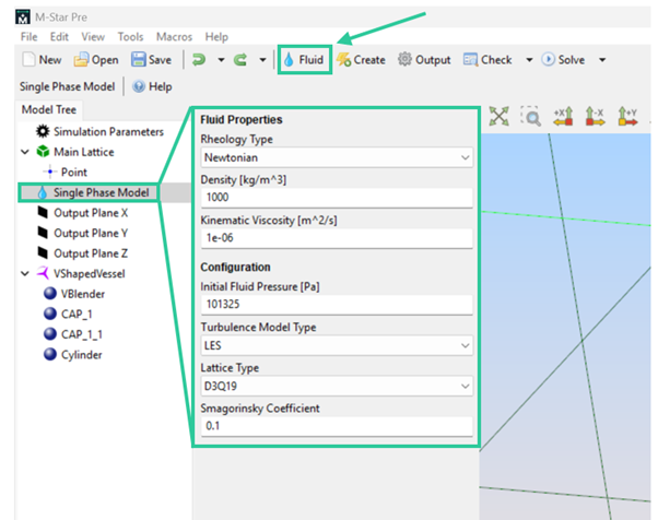
Fluid modelling: settings and Fluid menu location.

To set up the fluid, we select the Single Fluid Model in the Model Tree. The Information window appear, and we introduce the fluid properties for air:

• Rheology type -> Newtonian

• Density (kg/m3) -> 1.225

• Kinematic viscosity (m2/s) -> 1.460e-05

The remaining parameters stay as they are, with a pressure corresponding to sea level, large eddy simulation to resolve the turbulence, D3Q19 lattice (for our type of simulation 19 velocity directions is enough to properly resolve the problem) and the Smagorinsky Coefficient = 0.1 (a coefficient required for LES simulations set by default to 0.1, values obtained from predictions using direct numerical simulation).

With the fluid defined, we need to identify which area of the fluid domain we want to simulate. The current geometry set up splits the domain in two separate volumes: the air inside the vessel and the air outside the vessel. Clearly, we are just interested in what happens inside the vessel, so to define the flow domain we go to Main Lattice section in the Model Tree -> Below we can see a child point. This point appears on the geometry as a pink element and it works as follows: M-Star will compute the simulation in the volume the point is sitting, so, we need to move the point inside the V-shaped vessel (see image below).

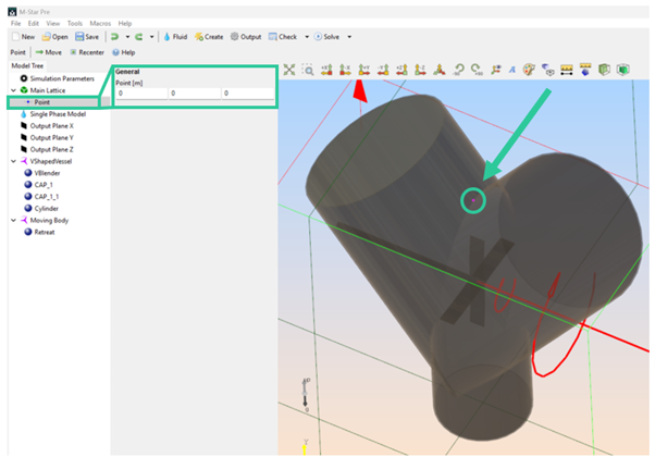
Main Lattice point: definition and geometry display.

To locate the point inside the vessel, just modify the point position by inputting the coordinates on the interactive window, you can see how the point changes its position. For this example, the coordinates (0, -0.364, 0) would work.

To finish with this section, we need to check the bounding box definition to make sure all the geometry will stay inside it. While this is trivial form many cases, the model we are setting up currently has a special approach as all the fluid domain moves, we must ensure that for all the positions along the simulation all the geometry stays inside the bounding box. As well, it is recommended to adjust as much as possible the bounding box to the geometry. The bounding box can be adjusted automatically:

Right click on Main Lattice -> Reset

But this approach can be inefficient and sometimes wrong, hence it is recommended to use a manual adjustment. Below we can see the default bounding default bounding box created by M-Star and the adapted version.

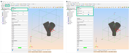
Model bounding boxes: default automatic and user defined.

As it can be seen, the modified bounding box is more centred on the geometry and tightly fitted to the vessel.

There are two options to manipulate the bounding box:

• Main Lattice -> Edit box (on the upper menu): this allows us an interactive manipulation of the box by dragging control points.

• Domain Mode -> Custom: enables modify the box by modifying the coordinates of the points that define the box.

Particles set up

Once the geometry (and its kinematics are defined) and we set the fluid environment, we are ready to set up two powder compounds, modelled as DEM particles.

When creating new DEM particles (and other M-Star features) we have two different steps: define the particles properties and create the injection geometry. For now, let’s create the DEM particles:

Go to Create -> Particles -> DEM Particles

A new window will pop up to define the injection geometry. This could be skip for now. Rename the DEM Particles we just created:

Select DEMParticles in the tree -> Right click -> Rename -> Change the name in the pop-up window to RodentFeed1 (or preferred name).

Good Practice

Remember: it is good practice to name properly all the different components in the model, this will allow us to keep models tidy and well organized, making things easier for future uses, modifications and post processing.

Now, we will define the particle properties using the powder characteristics provided and other considerations derived from the problem presented.

Click on RodentFeed1 in the tree, the options related to this object will appear in the Property grid, between the tree and the viewer panel.

Particle properties definition: Property grid

In the property grid select:

• Injection option -> Total Mass

• Injection location -> Child volume

• Total mass value (kg) -> 1.8 (data provided)

• Dump time UDF -> 0.0 (we start to release the powder for the first component as soon as the simulation starts)

• Density (kg/m^3) -> 500 (data provided)

• Volumetric Generation -> Off (for this case, we do not want new particles to be created as the simulation run).

• Initial size distribution -> Distribution type -> Single (this indicates that all the powder particles are the same size; other options are available to define the particle distribution: uniform, normal, etc. Toggle in the drop-down menu to check the options, M-Star online documentation can provide further insight).

• Diameter (m) -> 0.005 (this value differs from the data provided, however as mentioned earlier, we will perform a particle size sensitivity study for mixing and it is recommended start with large particle values and iteratively reduce this value until we reach a mixing condition independent of the particle size).

• Forces and Fluid Coupling -> Representation -> Unresolved (as particles are smaller than the lattice spacing, force interactions are resolved using empirical correlations. This is the approach used on most CFD-DEM simulations. Resolved approach is also available, however very fine mesh is required for this modelling as particles must be large compared with the grid size requiring large computational resources.)

• Gravity force -> On (powder particles are affected by gravity)

• Virtual mass -> On (powder particles are affected by the virtual increase in effective mass of a particle when moving through a fluid)

• Lift Saffman -> Off (powder particles are not affected by the lateral lift force generated by the particle rotation; typically, neglectable)

• Drag Force -> FreeParticle (powder particles are affected by the drag force modelled using the free particle approximation).

• Two-way coupling -> Disabled (the particles are small and the fluid dynamics do not affect the mixing problem).

• Fluid-Particle Force UDF -> leave it blank (this area can be used to define any forces acting in the particles).

• Moving body interaction -> BounceSimple (the particles will bounce back with interacting with the solid bodies from the model. Apply this to all the solids in the model individually).

• Particle-particle interaction -> Interaction type -> Hertz Contact (the particles would interact to each other using Herz model. Leave all the remain options on this section as the default values as they are the typical ones to model most of particle interactions.

• Breakup/Coalesce -> Off (we are not considering the powder particles to breakup under the external forces suffered along the simulation)

• Coalesce enables -> Off (it is assumed that the powder particles wouldn’t join due to the interactions between pairs of particles).

• Advanced -> Injection Downsampling -> 1 (parameter to reduce the number of particles input in the model via tracking them as parcels with the objective of reduce the memory requirements of the simulation, it is especially important in large vessels. It is recommended keep this parameter as low as possible (1 or close to 1) to avoid graining or under sampling. Using Injection downsampling=1 means that no parcelling is performed, and that would be our setting: however, if it is required to do so it is recommended keep the parcels withing the order-of-magnitude consistent with the lattice count).

• DEM bounce method -> Triangle (defines the particle interactions with the solids; triangle means that the interaction would be with the triangles from the tessellation of the static bodies. It is more realistic than Cell option as particle trap is avoided, but computationally more expensive).

• DEMCutoff dyameter -> 0 (all particles would be treated as DEM, decision based in the fact that all particles are the same size and it wouldn’t change along the simulation. If different particle size, this option would allow to treat some of them, the ones below the threshold diameter, as inertial particles, reducing the computational requirements).

• Initial Velocity type -> Constant (powder particles would be introduced at a constant velocity, no forced acceleration)

• Initial velocity -> x = 0, y = 0, z = 0 (particles are dumped in the vessel from a static condition)

• Compute Nearest Neighbour Distribution -> On (the simulation will compute average nearest neighbour separation distance and nearest neighbour separation distance, useful to characterize particle dispersion).

• Enable Particle Freezing -> Off (we do not want to fix particles in space at any specified time).

• Enable movement control -> Off (enables a user defined function to control if the particles move or are frozen. We have it disabled as we want the particles to always can move).

• Compute pressure gradient force -> Off (for this type of movement, we do not require to calculate the pressure forces over the particles, it is assumed to be neglectable).

• Enable Removal UDF -> Off (if active, allows to remove particles based on user defined laws).

• Enable Wall Hertz model -> Off

Once we have characterized the particles we must define from where they are injected (we already specify how in the section above) -> we have to create the injection geometry.

As we defined the injection location as Child volume, we must create that volume and assign it as an injection location.

To create a child geometry for a DEM particle, go to the tree:

Select RodentFeed1 -> right click on it-> Add geometry -> Parametric -> Primitive -> Cylinder -> OK

A new cylinder would appear on the screen. Now, we need to position in the location from where we want the RodentFeed1 powder to be released and adjust its size:

Position the cylinder using the tool Mate.

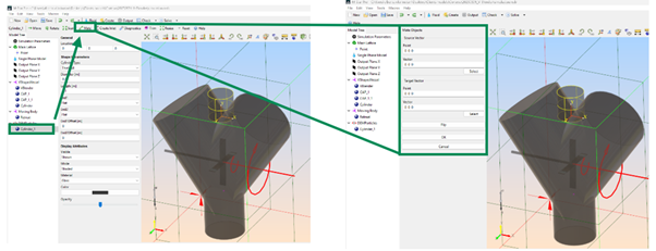
M-Star Pre Mate tool

For source vector click on “Select” and select the cylinder bottom edge. Click “Finish” when done. In Target Vector click on “Select” and select the top edges of the left side arm of the V-shaped vessel. Click on “Finish” to accept the selection. A wireframe representation of the cylinder would appear on your screen showing how it would look in the new position. Use the button “Flip” to modify the direction and make sure the cylinder would be inside the vessel, if needed. Once happy with the result, click “OK” -> The cylinder solid geometry would be displayed now on the new location.

Adjust the cylinder: We must be careful and make sure the geometry defined is big enough to house all the DEM particles. If the volume defined is too small, it would cause problems.

To know the cylinder dimensions, first we want to match the injection geometry (the cylinder) to the inlet at the top of the V-shaped vessel: hence the radius would be the same. Use the tool Measure Point to Point (see below).

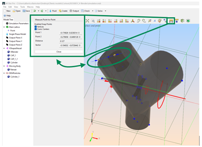
Point to point measurement

The result is 0.127 m, exit the measurement tool and Select the Cylinder in the tree. Define the Cylinder diameter as 2x0.127 m.

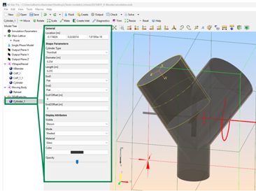
Injection cylinder definition

Now, we need to find the cylinder length, for this we will use some data that we already have. We know that the mass of RodentFeed1 is 1.8 kg and its density is 500 kg/m3; which means that the total volume required is 0.0036 m3. However, we are modelling the powder as spheres and it is well known that packing them in any shape leaves gaps, hence, to ensure good packing the cylinder volume should be bigger. Based on some literature, a good safe factor would be doubling the cylinder volume (as a rule of thumb), which means that the overall cylinder would be 0.0072 m3. With this in mind, and using the cylinder radius, the cylinder length is ~0.150 m. For this particular case, this cylinder would be still too small creating an error as the DEM particles would overlap each other. After an iterative process it was found that a cylinder length of 0.255 m would solve this issue, this represents a volume ~3.6 time bigger than the one calculated via powder mass and density.

Repeat the complete particle setting up for the seconds powder compound (AI Feed 2) considering:

• Dump time -> 2.5 seconds

• Total mass -> 0.063 kg

• Density -> 688 kg/m3

• Particle diameter -> 0.00438 m (apply a scale factor to achieve the same relative size between the two DEM particles as the one provided in the problem definition)

• Create a valid injection geometry based on the data provided and the recommendation suggested above.

Mixing index set up

As we discuss earlier, we will use entropy of mixing as mixing index to characterize the degree of “mixingness”. Remember the equation:

\[S = \frac{1}{S_0} \sum_{i} (x_1(i,j,k)\log(x_1(i,j,k)) + x_2(i,j,k)\log(x_2(i,j,k))) \frac{N_{cel}(i,j,k)}{N}\]

To implement it, we can follow the steps listed below:

Let’s start by obtaining the total number of particles in the whole domain:

Create -> Global Variable

A global variable is a single value that is globally available in all user defined functions.

Rename the global variable as rodentFeedTotal and select the following options:

• Data source -> Particles

• Data source particle name -> RodentFeed1

• Reduction -> Sum

• Global variable UDF -> Edit -> value = 1;

The above definition will allow us to quantify all the particles in the whole volume domain (the reduction operation delivers a single value from multiple inputs, in this case represent the number of particles for the RodentFeed powder).

Repeat the process for AIFeed.

We can use Global variables to create placeholders for variables (or as a way to declare new variables that will be computed in the whole domain). For example, currently we need to define a variable N that represents the total number of particles in the control volume, this variable N is the addition of both global variables defined above, basically: N=rodentFeedTotal+AIFeedTotal. So first we need to introduce the variable N:

Create -> Global variable

Now rename the variable as N and set Data source ->None. This will leave the variable empty, ready for being used.

However, we want N to represent the total amount of particles: we have to define this via a Custom script:

Create -> CustomScript

Rename the script as NCalculation and in the edit panel type:

void timestep(double t, double dt)
{
    N=rodentFeedTotal+AIFeedTotal;
}

This calculation would be executed each time step.

The next step is to define the number of particles on each voxel; we will use fluid variables for this purpose. The fluid variables are applied on the entire domain and evaluate any defined variable or parameter on each cell, delivering custom fields based on the provided inputs.

Let’s start by defining the number of particles of rodent feed on each voxel:

Create -> Fluid Varialble

Rename the variable as Ncell_1 (for simplicity and keep the same convention as the equation provided above)

Now, let’s define this fluid variable, change the following inputs:

• Calc Type -> Particles (we want to quantify the number of particles on each cell)

• Particle set -> Rodent Feed1

• Reduction type -> Sum (we want to know how many particles we have on each voxel.

• Custom Variable UDF -> Edit -> type: value=1; (we want that each particle counts as one)

Repeat the above for Ncell_2 (assigned to AIFeed2).

As well, we want to know the total number of particles on each voxel, so for this we will use fluid variables again:

Create -> Fluid variable

Rename it as Ncell_total and change the options as shown below:

• Calc Type -> cell (the parameters that we are going to use, Ncell_1 and Ncell_2, are already defined in the cells)

• Custom Variable UDF -> Edit -> Ncell_total=Ncell_1+Ncell_2; (we define the total particles in a cell as the sum of each species on each cell).

Tip

make sure the name of the fluid variable and the name used in the custom variable UDF are the same, if not M-Star will arise an error and fail when computing the parameter.

All we have defined so far are the building block to define the different elements of the equation shown above. When scripting an equation, it is recommended (and a best practice) to think on all the inputs that you will require and define a “plan” to design that output you want to obtain. This will allow you to have a more organized model, easier to understand and better to manage.

As said, we will start to build the different elements of the equation shown above; starting by x1 and x2: as those are quantities we want to evaluate on every single voxel of the whole domain, we will use fluid variables to do so:

Create -> Fluid variable

Rename it as x1 and modify the following entries:

• Custom Variable UDF -> Edit -> x1=Ncell_1/Ncell_total; (the fraction of particles in each cell is the number of particles of the species divided by the total number of particles on that same cell).

Repeat for x2.

Using the data provided above, we can assess the main term of the equation on each control volume cell using again a fluid variable. Once this is defined, we can compute the summation using a global variable. Let’s break this down:

Create -> Fluid variable

Rename it as localTerm and modify define the Custom variable UDF as follows:

localTerm=0;
if(x1>0&&x2>0&&N>0){
    localTerm=(x1*log(x1)+x2*log(x2))*Ncell_total/N;
}

Make sure the code doesn’t have any term divided by 0, as that will make the system fail (that is the reason why we put the conditional if in place).

Now we have the term defined in each voxel of the volume, which means we can apply the summation to all of it:

Create -> Global Variable

Rename it as totalEntropy and defined as shown below:

• Data source -> Fluid (the data on localTerm is a variable stored on each voxel)

• Reduction -> Sum (we want the summation of all values)

• Global variable UDF -> Edit -> value = localTerm; (we must to define what parameter we want to calculate)

This last global variable will measure the total entropy for the particles mixing, however…. We still need to normalize it using S0.

By definition S0 is the entropy of a completely mixed system. We can imagine this situation as a single cube where all our particles (both for RodenFeed and AIFeed) are enclosed.

Under the above consideration, \(N_{cel\_total} = N\), \(N_{cel\_1} = \text{rodentFeedTotal}\) (total number of partciles for the RodentFeed powder) and \(N_{cel\_2} = \text{AIFeedTotal}\). Applying those we get the followibg expression for S0:

\(S_0 = x_{1\_0}*\log(x_{1\_0}) + x_{2\_0}*\log(x_{2\_0})\)

Where \(x_{1\_0} = \text{rodentFeedTotal}/N\) and \(x_{2\_0} = \text{AIFeedTotal}/N\).

Once we have a clear idea on what we have to do, let’s define those variables: we want to obtain a number that represent the whole domain, hence we require a Global variables. We will define x1_0, x2_0, and S0 as empty global variables and perform the calculations using a custom script (same we did to calculate N).

Create -> Global variables

Rename the variable as x1_0, leave all the global variables as they are; make sure Data Source is set to None.

Repeat the process for x2_0 and S0.

We have declared all the new variables, and we can proceed to the calculations:

Create -> Custom Script

Rename it as S0Calculation and click on Edit. Type the following:

void timestep(double t, double dt)
{
x1_0=0;
x2_0=0;
S0=0;
if(rodentFeedTotal>0&&AIFeedTotal>0&&N>0){
    x1_0 = rodentFeedTotal/N;
    x2_0 = AIFeedTotal/N;
    S0 = x1_0*log(x1_0) + x2_0*log(x2_0);
}
}

Now we have S0 calculated and stored as a global variable.

The last step is normalizing the total entropy we have calculated before using S0, for doing this we will create a new global variable to store this new variable, and we will calculate it using a custom script.

Create -> Global variable

Rename it as totalEntropy_normalized. Leave all the settings as default, make sure Data source is set to None.

Create -> Custom script

Select Edit and define the normalized entropy as follow:

void timestep(double t, double dt)
{
    totalEntropy_normalized = totalEntropy/S0;
}

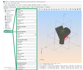
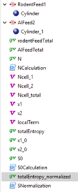
Once all the above variables are created, your model tree would look like the image below:

Model tree with the variables required to calculate the mixing index.

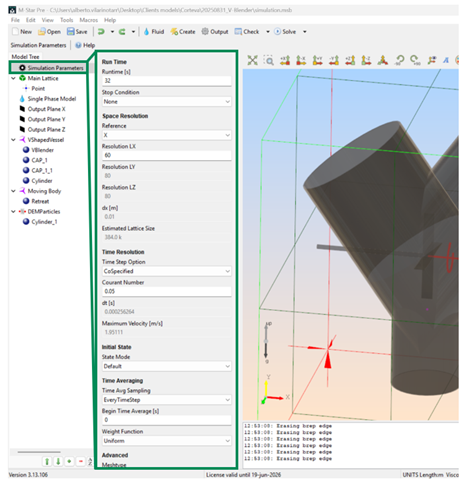
Simulation parameters set up

As final step, we must check and adjust the simulation parameters (spatial refinement, time step size, etc.) for our simulation.

Select Simulation Parameters on the Model Tree.

Simulation Parameters menu

Change the following parameters:

• Run Time (s) -> 32 (discussed earlier, this is the total simulation time we want to execute)

• Stop Condition -> None (run the simulation until the end)

• Space Resolution -> Reference -> X (use this direction to define spatial refinement)

• Resolution LX -> 60 (60 division in x direction; Y and Z will update automatically. These settings deliver a mesh size of 0.01 m, quite coarse but aligned with the DEM particle size. When reducing the particle diameter for the sensitivity study adjust accordingly).

• Time Resolution -> CoSpecified -> Courant Number -> 0.02 (this setting delivers a time step of 0.000206s, enough ensure a stable simulation with the spatial resolution defined. As we define the time step via Courant number, it would adapt as we modify the spatial resolution; however, sometimes we would require modifying the Courant number to keep guaranteeing the simulation stability).

• DEMTime Step Option -> Custom (this option allows us to decouple the DEM time step from the fluid time step, usually DEM particle require different time steps than the fluid resolution, and set the DEM time step manually to achieve the best balance between efficiency and resolution.)

• DEMTime Step -> 0.0001 (set the DEM time step to guarantee a stable simulation from the particle simulation point of view; if the particle size changes the DEM time step must change accordingly).

Now, we are ready to run the model. Save the simulation case (it is recommended to do periodical savings) and click “Solve” to launch M-Star Solve and execute the simulation.

Post processing

Open M-Star Post, you would be able to visualise the simulation time evolution, interrogate the flow and particles movement, etc.

As well, under “Global Variables” you can visualize the parameters we created. Isolate totalEntropy_Normalized and you can visualize the Mixing Index time evolution (see below).

Mixing Index time evolution

The graph shows the mixing evolution, a perfectly mixed system should show S=1; this level of mixing can be difficult, or impossible, to achieve and what we are interested in observing is if the curve flattens indicating that a stable state has been achieved. In the image above we can see that this situation has been achieved at t~30s indicating that the proposed time is enough to achieve a stable state.

Now, as we used quite large particles the maximum value of this index can change depending on the particle size. It was explained earlier that we must run different simulation with different particle size, find the maximum mixing index for each particle configuration and compare it across different particle sizes to check at what particle diameter value the mixing index stays constant.

To support the above, and from a data uniformity perspective, we will take the convention that the characteristic mixing index for each simulation is the one achieved at the very end of the simulation (t=32 seconds) and the simulation characteristic particle size would be the one corresponding to the RodenFeed1 particles. To obtain the mixing at t=32, we can place the mouse cursor on the graph and a small window will appear showing the data corresponding to that point; place the cursor at the very end of the graph and record the data for the Mixing Index. We can keep track of it, alongside the particle diameter, on an excel sheet.

Future work

Once the first simulation has run and we have a look at the output data, we must continue the particle size sensitivity study: re-run the simulation iteratively with smaller particle size each time, when setting up those models keep in mind:

• Change both compounds particle sizes (RodenFeed1 and AIFeed2), and make sure their relative size is respected.

• Adjust the simulation spatial resolution as required to maintain the ratio between grid size and particle size. Although, from a certain particle size the spatial resolution can stay the same as a too refined mesh can be unaffordable, keep an eye on the mesh size.

• If required, adjust the Courant number to guarantee the simulation stability.

• Adjust (reduce) the DEMTime step to ensure proper resolution for the particles.

• Post process all the simulations, extract their characteristic mixing index and track them alongside with the characteristic particle size. Once the mixing index becomes constant, it means we have found the particle size that makes independent the mixing properties and the results extracted from that model would be equivalent to those with smaller particle diameter (in our case 194 microns). This approach allows us to compute the simulation, model all the particles would be impossible to run, with the minimal resources possible while delivering a realistic and reliable result.

The particle size that flattens the curve on on the graph particle size vs. mixing index correspond to the simulation we should be using to answer the questions related with this problem.